Economic data currently is providing plenty of mixed signals to California’s policymakers, as they continue to craft state and local budgets in a constrained fiscal environment. California’s economy now is clearly improving in many important ways, including employment growth. Nevertheless, significant impediments block the state’s path to a more robust recovery from the recent, staggering economic downturn.
Like the economic data, reports concerning state revenues also have been delivering some mixed messages recently, with recent weakness in income tax payments accompanied by speculation concerning a future bonanza of tax revenues due to the possible initial public offering (IPO) of stock by Facebook, Inc. This report provides our updated projections concerning these and other trends in the economy and state revenues.
Job Growth and Economic Confidence Rising . . . Wage and salary employment has increased at a healthy clip in recent months in California and for the nation as a whole. This is one of the most tangible signs that the economic recovery from a staggering recession is picking up steam. Job growth appears to be helping business and consumer confidence, which helps retail and other sales.
. . . But Persistent Joblessness Remains a Key Problem. Despite the promising job growth news, California’s unemployment levels remain stubbornly high—worse than all other states except Nevada. Wide disparities remain among regional job markets, with coastal areas generally doing better than areas in the Central Valley and Inland Empire, and significant disparities in employment opportunity still exist among different age, racial, and ethnic groups. Perhaps most troubling is that the number of Californians unemployed for long periods has skyrocketed.
Housing Market Remains Very Troubled. Home prices nationwide are expected to slip further in early 2012 before hitting bottom sometime later this year. We expect construction–related employment in California—still at incredibly weak levels due in large part to the housing bust—to increase a bit in 2012 before beginning somewhat more robust growth in 2013. While these forecasts indicate some modestly promising trends in the housing market—particularly in the multi–family housing sector—the foreclosure rate still remains very high in some regions of the state. Depressed housing prices will remain a drag on the state economy for some time.
Corporate Profits and Technology Companies Have Been Booming. Despite persistent challenges that remain for the construction sector and some other businesses, aggregate corporate profits continue to grow sharply. This trend is exemplified by a California–based firm—Apple Inc.—that recently reported profits of about $1 billion per week during its most recent fiscal quarter and now ranks as the most valuable company in the world. Meanwhile, less than one decade after its founding, another California technology company—Facebook, Inc.—soon is expected to offer its stock in a highly anticipated IPO. Facebook’s possible IPO and IPOs of other California technology companies are likely to generate substantial capital gains and other income for a small number of Californians and, in so doing, generate additional state tax revenues over the next few years.
Federal Policy Important, but Much Uncertainty About the Future. Federal monetary policy, set by the Federal Reserve, has been significant in helping the recovery gain steam, but federal fiscal policy now is offsetting the monetary policy, as the federal government decreases spending levels. The future direction of federal tax and budgetary policy remains quite uncertain, with Congress and the President likely to make significant decisions regarding future tax levels and deficit reduction after the November 2012 elections. These decisions could affect the state budget significantly in the coming months and years.
Negative Trends We Identified in January Seem to Be Continuing. While the economic outlook has improved somewhat since our last forecast in November, data received after that forecast concerning 2010 tax payments by Californians and soft personal income tax (PIT) estimated payments in December and January have weakened some parts of our office’s near–term revenue forecast. In January, we noted that our November General Fund revenue forecast was $6.8 billion lower than the administration’s in 2011–12 and 2012–13 combined (including our lower estimates of revenue from the Governor’s proposed tax initiative). Now, our updated revenue forecast—including similar federal tax policy assumptions as the administration’s, an updated estimate of revenues from the Governor’s initiative, and an initial estimate of revenues due to the possible Facebook stock offering—is $6.5 billion lower than the administration’s in 2011–12 and 2012–13 combined. If the Facebook–related revenues were omitted from this new forecast, General Fund revenues would be about $8.5 billion lower than the administration’s over this period—weaker than the $6.8 billion difference identified in January—due mainly to the negative revenue data received over the last three months.
Effect on Budget Problem. If our revenue forecast proves to be more accurate than the administration’s, the Legislature and the Governor will have to identify additional budgetary solutions to bring the 2012–13 state spending plan into balance. (The net effect of our lower revenue assumptions on the near–term budget problem, however, will depend on how this updated forecast affects the Proposition 98 minimum guarantee for schools and community colleges. We expect to develop updated Proposition 98 estimates in the coming weeks.) Much more information will become available by the end of April, when a large amount of income tax payments are received by the state and refund payments are made. The Legislature will want to wait until after this data is analyzed in the May Revision process before making its 2012–13 budget decisions. We hope that the information provided in this update will help set the stage for the work of legislative budget subcommittees in addressing the state’s fiscal situation.
This report is divided into three sections:
Perspectives on the Economy. In the first section, we discuss the current state of the U.S. and California economies and recent major trends in each.
The Economic Forecast. In the second section of the report, we discuss the major elements of our updated, independent forecast of how the U.S. and California economies will perform over the next several years through 2016–17.
The Revenue Forecast. In the final section of the report, we discuss our updated forecast of state General Fund revenues through 2016–17, including an updated estimate of the revenue impact of the Governor’s proposed tax initiative, a key element of his proposed budget plan.
Economic Recovery Continues. The U.S. and California economies continue to recover from the recession that ended in 2009. After slowing through much of the summer as the European debt crisis and the congressional debt–ceiling debate worried financial markets, the U.S. economy rebounded late in the year, which sets the stage for more promising growth in 2012.
Despite Persistent Challenges, Consumer and Business Confidence Is Building. Households continue to face significant challenges—including limited growth in disposable income, stubbornly high unemployment levels, tight credit markets, and burdensome, although declining, mortgage debt. The number of individuals who have been unemployed for a prolonged period remains alarmingly high in California and other states. Each of these challenges dampens aggregate demand for goods and services, which, in turn, affects business hiring and production decisions. Recent strength in key economic data, however, suggests that consumers and businesses have become more confident about the course of the recovery, especially when compared to last summer. We expect this trend will continue and perhaps strengthen somewhat in the coming months.
Fourth Quarter of 2011 Showed Positive Signs. U.S. real gross domestic product (GDP) grew at an annualized rate of 2.8 percent in the fourth quarter, the most encouraging growth of 2011. Preliminary data from January suggests a continuation of this level of growth. A number of key economic variables are showing strength:
- U.S. and California Job Growth Has Been Picking Up. National wage and salary employment increased by 243,000 jobs in January, exceeding consensus expectations. Initial employment estimates for November and December also have been revised upward. On average, over the past three months, the U.S. economy added 201,000 jobs monthly. Favorable winter weather may have contributed to this trend. In California, nonfarm payroll employment increased by over 240,000 between the end of 2010 and the end of 2011, including monthly increases of 24,700 in November 2011 and 10,700 in December 2011.
- Retail Sales Are Increasing. Preliminary estimates indicate that retail sales are up 6.2 percent over the last three months, compared to the same three months one year ago. In January, retail sales (excluding gasoline and autos) increased sharply, with strong growth in general merchandise, department store, sporting good, and grocery sales. Online and mail order sales during the fourth quarter of 2011 improved 15.5 percent from 2010 holiday season levels, and online sales now account for over 5 percent of all such holiday sales. This trend has helped improve shipping and delivery employment in recent months. Despite recent rises in gasoline prices, consumers have been spending.
- Strong Recent Growth in Auto Sales. Sales of light vehicles (cars and small trucks) reached 14.1 million vehicles in January (annualized and seasonally adjusted), the strongest monthly sales since May 2008, excluding months affected by the “cash for clunkers” program in 2009. Domestic auto companies have shown strength recently, and Honda and Toyota each have begun posting year–over–year sales gains as the companies continue to recover from last year’s earthquake and nuclear disaster in Japan. The average age of cars and trucks on the road has risen to a record high of 10.8 years, and this has created pent–up demand that should support strong auto sales in 2012.
- Consumer Confidence Improving. Consumer confidence, which fell to recession lows throughout the summer months, has climbed in recent months to much improved territory according to the Reuters/University of Michigan Consumer Sentiment Index, which measures consumers’ attitudes about the economy and their personal financial situation.
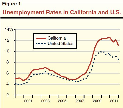
State Unemployment Rate Stubbornly High, but Falling. As of December 2011, California’s unemployment rate is 11.1 percent. Compared to other states, California has a high unemployment rate and a correspondingly very weak job market. Currently, only Nevada has an unemployment rate that is higher than California’s. During and after the recession, the trend in California’s unemployment rate generally followed the same basic trend as the national unemployment rate, as shown in Figure 1. California’s unemployment rate was about 4.8 percent at its most recent low point in late 2006. It peaked at 12.5 percent in late 2010 and has since fallen to 11.1 percent as of December 2011.
Wide Job Market Disparities Throughout the State. Some regional labor markets in California have done significantly better or worse than the state as a whole. Figure 2 illustrates this and shows that the recession continues to affect the state’s regions to varying degrees. As discussed above, the statewide unemployment rate remains 6.3 percentage points above its pre–recession low. Statewide, about two–fifths of the state’s Metropolitan Statistical Areas (MSAs) currently have unemployment rates that are 6 or fewer percentage points above their pre–recession low. Los Angeles County and Orange County combined have an unemployment rate that is 6.6 percent above its pre–recession low. For another two–fifths of the state’s MSAs, however, unemployment remains 7 or more percentage points above the pre–recession low, ranging from the Hanford–Corcoran MSA (Kings County) at 7.2 percentage points above the pre–recession low to the Yuba City area (Sutter County and Yuba County) and El Centro (Imperial County) at 9.1 and 13.7 percentage points, respectively, above their pre–recession lows. Thus, while labor market conditions generally are improving, they are improving from a very dire state in many areas of California. Despite the improving economy, this means that many Californians will continue to face troubling wage and employment prospects for the foreseeable future.
Figure 2
Recession Affected State’s Labor Markets to Different Degrees
|
Metropolitan Statistical Area
|
Labor Force at
End of 2011
(In Thousands)
|
Previous
Minimum Unemployment
Ratea
|
Unemployment
Rate at End of 2011
|
Percentage
Point Change in Unemployment
Rate
|
|
El Centro
|
77
|
14.6%
|
28.3%
|
13.7%
|
|
Yuba City
|
71
|
8.7
|
17.8
|
9.1
|
|
Merced
|
106
|
9.2
|
18.0
|
8.8
|
|
Stockton
|
298
|
7.3
|
15.8
|
8.5
|
|
Fresno
|
434
|
7.7
|
16.0
|
8.3
|
|
Modesto
|
235
|
7.8
|
16.0
|
8.2
|
|
Riverside/San Bernardino/Ontario
|
1,775
|
4.8
|
12.8
|
8.0
|
|
Madera/Chowchilla
|
66
|
6.8
|
14.5
|
7.7
|
|
Redding
|
85
|
6.4
|
13.9
|
7.5
|
|
Visalia/Porterville
|
211
|
8.4
|
15.7
|
7.3
|
|
Hanford/Corcoran
|
62
|
8.1
|
15.3
|
7.2
|
|
Bakersfield/Delano
|
372
|
7.4
|
14.3
|
6.9
|
|
Chico
|
104
|
6.0
|
12.7
|
6.7
|
|
Los Angeles/Long Beach/Santa Ana
|
6,459
|
4.3
|
10.9
|
6.6
|
|
Sacramento/Arden–Arcade/Roseville
|
1,031
|
4.6
|
11.2
|
6.6
|
|
Vallejo/Fairfield
|
213
|
4.8
|
10.8
|
6.0
|
|
Santa Cruz/Watsonville
|
152
|
5.5
|
11.3
|
5.8
|
|
Salinas
|
217
|
6.7
|
12.5
|
5.8
|
|
San Diego/Carlsbad/San Marcos
|
1,583
|
3.9
|
9.3
|
5.4
|
|
Santa Rosa/Petaluma
|
252
|
3.9
|
9.3
|
5.4
|
|
Oxnard/Thousand Oaks/Ventura
|
432
|
4.2
|
9.5
|
5.3
|
|
San Luis Obispo/Paso Robles
|
135
|
3.9
|
9.1
|
5.2
|
|
San Francisco/Oakland/Fremont
|
2,244
|
4.1
|
8.9
|
4.8
|
|
San Jose/Sunnyvale/Santa Clara
|
918
|
4.5
|
9.3
|
4.8
|
|
Napa
|
74
|
3.7
|
8.5
|
4.8
|
|
Santa Barbara/Santa Maria/Goleta
|
220
|
4.0
|
8.6
|
4.6
|
|
California
|
18,219
|
4.8%
|
11.1%
|
6.3%
|
|
United States
|
153,887
|
4.4
|
8.5
|
4.1
|
In addition to these regional disparities in unemployment, disparities among California’s racial, ethnic, and age groups also persist. In December 2011, the unemployment rate reported for African Americans was 19.6 percent, and this rate was at 13.8 percent for Hispanics and 8.9 percent for Asian Americans. For whites, the unemployment rate was 11.3 percent. By age group, the unemployment rate is higher for Californians aged 16 through 19 at 35.2 percent and for those aged 20 through 24 at 17.6 percent. By contrast, the jobless rate for those aged 35 through 44 is 9.3 percent and for those aged 45 through 54, 10 percent.
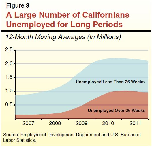
Alarming Level of Long–Term Unemployment in California. Finding a job typically takes time. Weaker economic conditions can make job searches even more difficult and time–consuming. At the end of 2011, the number of unemployed people in California still looking for work after more than 26 weeks accounted for 43 percent of the unemployed nationwide and 46 percent in California. This massive growth of California’s long–term unemployed since 2009 is shown in Figure 3. Even more troubling than this statistic is the fact that while the number of California’s unemployed for 27 to 51 weeks declined in 2011 (from 321,000 in December 2010 to 246,000 in December 2011), the number of those unemployed for 52 weeks or more increased (from 704,000 to 718,000). Now, more than one–third of California’s unemployed has been unable to find work for over one year.
Participation in the Labor Force Relatively Low, but Seems to Be Improving. Because being counted as “unemployed” in government statistics requires a person to be looking for work, people who have given up on looking for work are not counted when calculating unemployment rates or in the ranks of the long–term unemployed. For that reason, a different statistic, the labor force participation rate, can give a fuller picture of labor market conditions. The labor force participation rate is the percentage of the adult civilian population that is in the labor force. As of December, this rate was 63.4 percent in California and 64 percent for the U.S. as a whole. It has not been so low for the U.S. since the early 1980s or for California since 1977. In California, the labor force participation dipped below 63 percent during parts of 2011, but began to improve steadily late in the year. During 2011, it is estimated that a growing percentage of Californians aged 20 to 24 and 55 and over returned to the labor force. This offset estimated declines in labor force participation for those aged 16 to 19 and 25 to 54.
Why Discouraged Workers and Long–Term Unemployment Are a Major Problem. All of these trends have important implications. The fact that more people are unemployed for longer and that large numbers of people have opted out of the labor market altogether means that there is a significant population that may face permanent difficulties in reentering employment. Such individuals may have lost skills or connections they had or be unable to keep up with advances in business practices and technology. California governments, families, and nongovernmental organizations all will have some higher costs in future years to help support these individuals. This, in turn, may impair future economic growth to some extent.
Prices Outpace Disposable Income. Real disposable income declined slightly in the U.S. in 2011 as prices for consumer goods and services—such as fuel, housing, food, health care, and household services—grew more quickly than after–tax incomes. Real consumer spending, on the other hand, increased by 2 percent in 2011, propelled by pent–up demand for large items like vehicles and household appliances. Figure 4 shows the quarterly growth in real personal consumption expenditures—a measure of how much income earned by households is being spent on current consumption as opposed to being saved for future consumption.
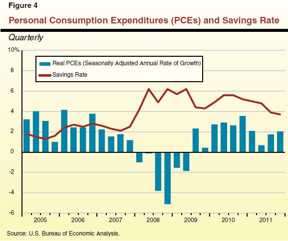
Savings Rate Declines Somewhat. As also shown in Figure 4, the U.S. savings rate fell from 5 percent to 3.7 percent over the course of 2011. Savings rates (savings as a percentage of disposable personal income) tend to decline during periods of strong economic growth, as income gains allow consumers to spend a larger portion of their income on goods and services, especially expensive discretionary purchases like vehicles, household appliances, and personal travel. On the other hand, savings rates tend to increase during recessionary periods as households pull back on discretionary consumption.
The recent trend toward lower savings rates may be the result of improved consumer confidence and a precursor to more robust spending in the near term. We remain cautious, however, because real disposable income was flat in 2011.
Lending Remains Relatively Tight. Availability of new consumer credit declined precipitously during the 2008 and 2009 financial crisis. Although lending restrictions loosened somewhat in 2011, many households continue to have difficulty acquiring home loans and other credit. This in turn has hurt the housing market, as stringent credit conditions seem to be keeping some willing buyers out of the market and limiting the ability of consumers to refinance at lower rates. According to the Federal Reserve, fewer than half of lenders are offering mortgages to borrowers with a credit score of 620 and a 10 percent down payment, despite such loans being within standard credit eligibility parameters. In general, the share of mortgage loans supported by federally related entities (primarily Fannie Mae, Freddie Mac, and the Federal Housing Administration) has increased significantly since the housing bubble collapsed, reflecting a general inability or unwillingness of private lending institutions to extend credit.
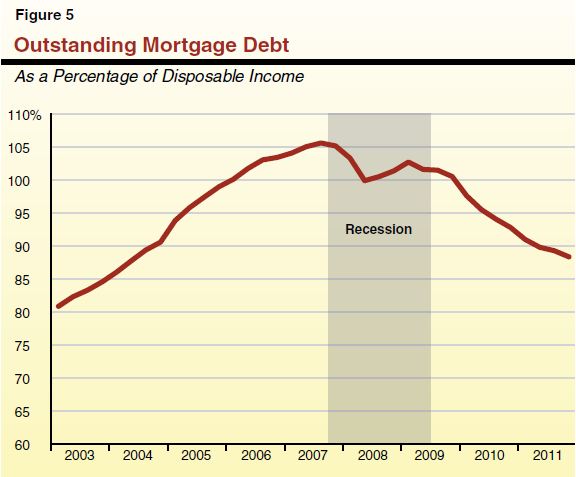
Reduced Mortgage and Non–Mortgage Consumer Debt. As shown in Figures 5 and 6, outstanding mortgage and non–mortgage consumer debt both have declined in recent years as a share of disposable income. (Non–mortgage consumer debt consists primarily of credit cards, student loans, and auto loans.) The decline in outstanding debt results largely from: (1) charge–offs, where consumer defaults (or foreclosures, in the case of mortgage debt) reduce personal financial liabilities, and (2) deleveraging, where consumers borrow less and pay off existing debt more quickly. Recent data show that although charge–offs have reduced debt levels somewhat, the bulk of the decline is attributable to consumers paying down mortgages and other forms of debt. Therefore, the majority of the decline in outstanding debt is the result of voluntary changes consumers have made to their spending and savings habits as opposed to their inability to meet financial obligations.
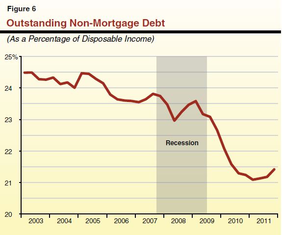
Outstanding non–mortgage debt as a share of disposable income remained relatively flat in 2011, as shown in Figure 6. Recent data indicates consumers may be expanding their use of credit cards and other non–mortgage debt. This is somewhat encouraging since the trend indicates that consumers have become more confident in their personal financial situation. Nevertheless, some caution tempers our optimism, since consumers may be shifting to credit use to spend at levels that may not be supportable by their future income gains.
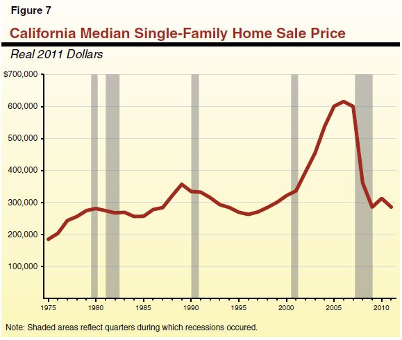
The U.S. and California economies continue to be weighed down by the housing market—including foreclosure activity, construction sector employment, and declining home values. California’s median home sale price, shown in Figure 7, has declined precipitously from pre–recession “housing bubble” levels. Home prices nationwide are expected to slip further in early 2012 before hitting bottom sometime during the second quarter of this year. Given the surplus stock of single–family homes and generally weak demand for housing, we expect construction–related employment in California to increase only marginally in 2012 before beginning more robust growth in 2013 and 2014.
Foreclosure Activity Has Multiple Effects on Households. The value of outstanding U.S. mortgages peaked at $11.1 trillion in the fourth quarter of 2007 before falling to $10.2 trillion in the fourth quarter of 2011. A portion of this decline is attributable to foreclosure activity. Home foreclosures affect household financial behavior in a number of ways:
- Following foreclosure, households often move into single– or multi–family housing (such as apartments, condos, or new single–family residences) that tends to be less expensive than their previous housing. Reduced housing expenditures, relative to pre–foreclosure levels, may free up spending for other goods and services. (Recent evidence suggests that relatively few households move in with friends or parents following foreclosure.)
- Over the longer term, however, mortgage defaults reduce consumer creditworthiness, which tends to increase the cost of future borrowing. To the degree that future borrowing becomes more expensive, households may reduce spending on other items or borrow less, both of which reduce consumption. The net impact of these two effects on households is unknown, but likely negative.
The Recession Has Delayed Household Formation. Household formation occurs when young adults move out of their parents’ homes or when individuals that share housing (either couples or non–related persons living together) move into separate units. During the recession, household formation declined as fewer young people moved out on their own or households combined in order to reduce housing costs. Delayed household formation has reduced demand for single– and multi–family housing, depressing real estate prices further.
In the Near Term, Delayed Household Formations May Favor Multi–Family Construction. Individuals that have delayed household formation in recent years may soon begin to move out on their own or with others in larger numbers. Such persons may be more likely to rent multi–family housing than to purchase a home, due to generally weak job and income prospects, the difficulty in accessing credit, and, perhaps, lingering uncertainty about investing personal assets in real property. As a result, multi–family construction starts have been increasing to meet growing demand. In fact, multi–family housing permits (which represent new construction activity) exceeded those for single–family residences in 2011 for the first time in the decades for which we have recorded data. According to a report from the American Institute of Economic Research, if construction of apartment buildings continues to grow in this manner, “the housing market may take a radically different—and high–rise—shape” in the future.
Foreclosure Rate Moderating in State, but Remains High in Some Regions. As shown in Figure 8, foreclosure activity in California has fallen somewhat over the last couple of years, although approximately 155,000 homes began foreclosure proceedings in 2011. Data for 2011 may be skewed downward, however, because lenders may have withheld some foreclosure notices during the 16–month investigation leading up to the recent “robo–signing” foreclosure settlement, which was reached between numerous states (including California) and several mortgage companies.
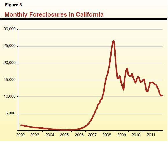
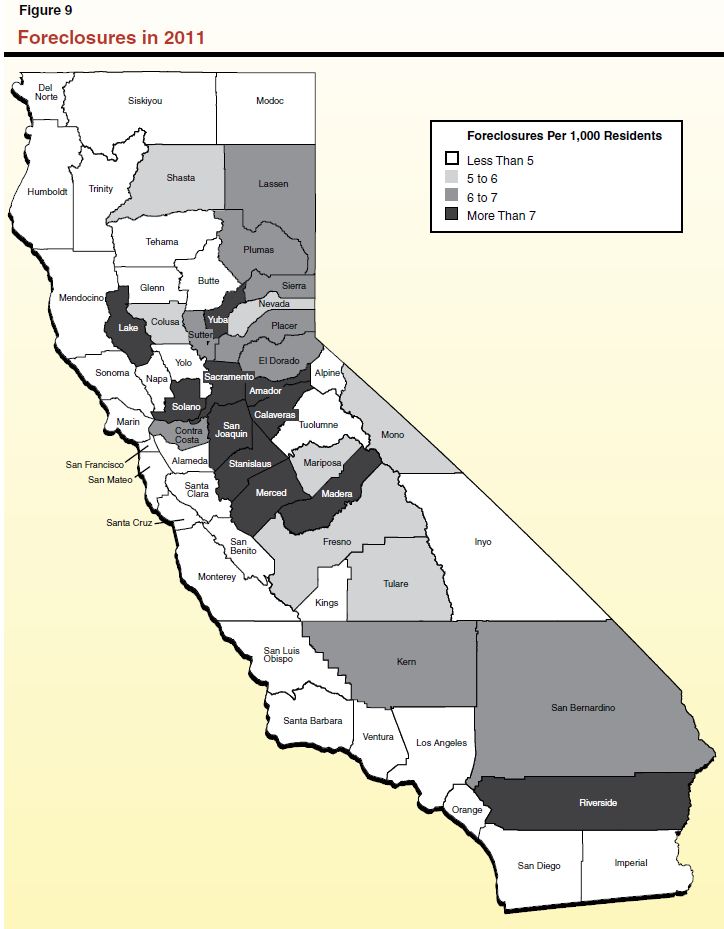
As shown in Figure 9, the frequency of foreclosures—measured by foreclosures per 1,000 residents—varies widely from county to county. Inland counties that experienced the most housing activity during the housing bubble seem to have been especially hard hit. Inland Empire and Central Valley counties have among the highest foreclosure rates in the state, and therefore, have experienced larger mortgage–related household spending changes than other regions. We expect foreclosure activity in California to continue, albeit at a declining rate, over the next few years. The rate of delinquent mortgage payments—a leading indicator for foreclosure activity—fell during the fourth quarter of 2011 to its lowest level since the housing market imploded.
Business Investments Increased Markedly in 2011. National business fixed investment—which includes purchases of tangible capital goods such as machinery, equipment, and software, as well as construction and expansion—grew 8.6 percent in 2011. Pent–up demand for investments that were deferred during the recession has led firms to retrofit facilities and purchase replacement equipment. On the other hand, high vacancy rates for commercial office space and generally weak expansion demand have prevented the commercial real estate market from improving much of late.
A subcategory of business fixed investment—business investment in technology, including software and computer systems—expanded 10.3 percent in 2011. These investments are especially important to California’s economy, which relies heavily on the professional and technology services sectors for high–wage employment growth.
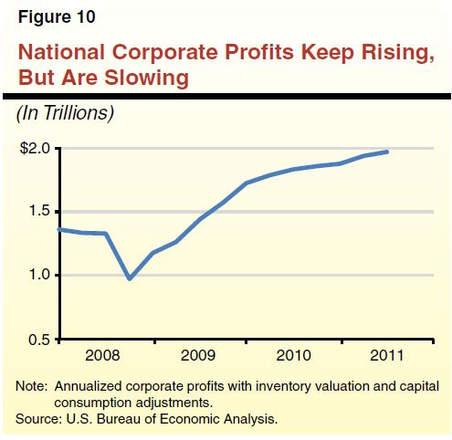
Corporate Profits Grew Strongly in Recent Years, May Now Be Slowing Somewhat. Corporate profits have rebounded dramatically from the recession, as exemplified by Apple Inc., which recently reported profits of about $1 billion per week during its last quarter. Growth in aggregate national corporate profits, however, has slowed recently, as shown in Figure 10. Slower growth in recent months may be the result of generally slower demand growth in international export markets, as well as a limited capacity to reduce production costs below their current levels.
Monetary Policy a Major Support for the Recovery. The Federal Reserve has continued its extraordinarily accommodative monetary policy recently by committing to near–zero interest rates through 2014 as well as continuing nontraditional monetary actions commonly referred to as “quantitative easing.” The Federal Reserve has a statutory mandate to foster maximum employment and price stability. In reaching its decision to pursue low interest rate policies for a very long period, the Federal Reserve’s Federal Open Market Committee has made the judgment—shared by the vast majority of economists—that continuing “slack” in labor market and other economic conditions has reduced substantially the threat of increased inflation in the near future. This reflects the Federal Reserve’s view that economic growth will be modest in the coming quarters and that unemployment will decline only gradually.
Federal Fiscal Policy Is Offsetting the Benefits of Monetary Policy. Aggressive federal monetary policy now is being offset somewhat by a decline in spending by the federal government. Specifically, the fiscal effects of the 2008 and 2009 federal stimulus packages have generally expired, and real federal government purchases of goods and services have declined since 2010. We expect this decline in federal outlays to continue as the nation’s leaders turn their attention more and more to addressing the federal government’s fiscal imbalance.
Federal Tax Policy and Temporary Unemployment Insurance Support the Recovery. Since 2011, the partial federal payroll tax reduction—coupled with the extension of emergency unemployment insurance benefits—has improved household financial conditions that face consumers. In particular, these federal actions have helped bolster consumer spending—which accounts for roughly 70 percent of GDP.
Uncertainties Regarding Future Federal Policies Cloud Forecast. California’s leaders will have to fashion a 2012–13 budget in the context of major uncertainty about future federal tax and spending policies. Considerable uncertainty about these policies likely will persist until after the November 2012 presidential election. One key element of the uncertainty results from the scheduled expiration at the end of 2012 of various tax cuts enacted under the Bush Administration (and extended under the Obama Administration), known informally as the “Bush tax cuts.” Another key uncertainty is how the federal government will reduce expenditures in coming years in order to implement its deficit reduction targets. In light of these and other federal policy uncertainties, our forecast must make a number of assumptions in these areas. Our economic forecast generally assumes the following:
- Payroll Tax Reduction and Unemployment Benefits. Consistent with recent legislation, our economic forecast assumes the partial federal payroll tax cut and certain emergency unemployment insurance benefits are extended through the end of 2012. In addition, our forecast assumes that these federal policy actions are phased out gradually after their currently scheduled expiration dates.
- Federal Deficit Reduction Legislation. Our forecast, consistent with that of many economists, assumes that automatic federal spending cuts set to begin under current law in 2013 generally will not proceed. Instead, our economic forecast assumes that Congress and the President will enact a compromise spending and revenue package to take effect beginning in early 2014. These measures are assumed to stabilize, but not reduce, the federal debt–to–GDP ratio.
- Bush Tax Cuts. The Bush tax cuts are assumed in our economic forecast to be extended an additional year to 2013. (This assumption is relevant for our PIT revenue forecast, as discussed later in this report. In our revenue forecast, we display different scenarios based on varying assumptions concerning the expiration date of the Bush tax cuts.)
Most economic forecasts—including our own and the administration’s—assume that Congress and the President agree to compromises in the coming months to mitigate some of the near–term negative economic effects that would occur if current law were left unchanged. The Congressional Budget Office estimates that real GDP growth under a fiscal policy scenario similar to that assumed in our forecast could be between 0.5 and 3.7 percentage points higher in 2013 than it would be if Congress and the President allow these changes to occur as scheduled. Over the longer term, however, the continuation of these near–term economic supports would likely result in the need for more significant tax increases and federal budgetary reductions than would be the case if these supports expired as scheduled.
Perhaps the most significant economic risks for this forecast relate to the unknown future direction of federal fiscal and tax policy, as discussed above. In this section, we discuss several other key economic risks and uncertainties.
Major Oil Price Spikes? Average statewide gasoline prices generally have been climbing since December. Our forecast assumes modest additional growth in prices through the middle part of this year, but international events threaten to cause supply disruptions that could result in significantly higher price spikes. Energy consumption equals a smaller percentage of American consumer spending than it did during much of the 1970s and 1980s, but spikes in gasoline prices, in particular, could hamper already fragile consumer confidence.
Tensions between the international community and the government of Iran—the world’s third–biggest oil exporter behind Russia and Saudi Arabia—have led that country’s regime to threaten oil supplies. Additionally, oil supplies in Nigeria and Venezuela remain vulnerable to political shocks there, and Iraqi oil output continues to be susceptible to attacks by insurgents. Should Libya be able to restore oil output to levels achieved prior to its recent civil war, this could offset potential disruptions from Iran and other areas. In addition to these international issues, domestic events—such as fire that occurred two weeks ago at a major oil refinery in Washington—can cause gas price spikes. Finally, California’s ambitious greenhouse gas reduction efforts will also add upward pressure to energy prices here over the next few years.
A More Prolonged Housing Slump? Our forecast assumes that the California and U.S. housing markets begin a slow recovery from their recent depths, fueled in part (as discussed earlier) by new multi–family housing construction. It is possible, however, that the housing market could perform even more weakly than we assume in our very modest growth forecast. For example, housing prices could continue to decline slowly for one or more years beyond what is assumed in our forecast. A more prolonged housing slump of this type would reduce the growth of building permits and delay even more a return to growth for the state’s construction industry. Such a slump could erode further or impair growth of assessed valuations, which, in turn, would affect local government property tax revenues and requirements for the state to provide funding to school and community college districts. Consumer confidence also could be constrained by a prolonged housing market depression. Offsetting the possibility of such a slump are the recent reports of unusually strong price appreciation in a few California markets—most notably, the Silicon Valley—which has been attributed in part to recent and upcoming IPOs of stock for Internet companies, such as Facebook.
Deeper Problems Than Those Already Expected in Europe? Europe’s economy continues to suffer from the effects of its sovereign debt crisis, which has strained both financial institutions and governments, and contributed to general economic and labor market weakness there. Our forecast assumes that Europe entered recession in the fourth quarter of 2011 and that the Eurozone countries’ GDP will decline by 0.7 percent in 2012. California exports goods primarily to Mexico, Canada, and Asia (particularly China and Japan), but the Eurozone also is an important trading partner. If the European recession is deeper or longer than we assume due, for example, to more extended delays in resolving the continent’s sovereign debt crises, our forecast could be negatively affected in the coming months.
Overall, GDP growth in the U.S.’s major–currency trading partners is projected to remain positive at 1 percent in 2012—down from 1.7 percent in 2011, in part due to the European recession and slower growth in the Chinese economy. Chinese leaders—dealing with a construction “bubble” in their own economy—currently face a tough balancing act: how to let economic growth slow enough to contain inflation but not so much that it causes a “hard landing” for the economy. Offsetting the weakness in the Chinese economy is the likely resumption of moderate growth in the Japanese economy, which is recovering from last year’s earthquake, tsunami, nuclear disaster, and associated energy disruptions.
Economic forecasting—which relies on historical economic experience to help project how the economy will perform in the near future—has been subject to particular uncertainty in recent years. There is little precedent for a downturn of the magnitude the economy has just experienced. Accordingly, making sound judgments about how the economic recovery will proceed in the short term and the medium term presents unique challenges and requires us to acknowledge that significant economic risks and uncertainties remain.
Recovery Generally on Track With Expectations. The course of the recovery has been slower and more grueling than most economic estimates made in recent years, including our own. It appears now, however, that the economy is tracking fairly closely to our most recent economic forecast of November 2011. Growth continues to be held back by (1) lingering foreclosure activity and declining home values, as well as weak growth in real disposable income and (2) constrained spending by federal, state, and local governments. Figure 11 displays the key economic variables for our newly updated February 2012 economic forecast, and Figure 12 compares several of those key variables with assumptions from both our office’s November 2011 economic forecast and the administration’s January 2012 forecast (which generally was assembled before the start of the calendar year).
Figure 11
LAO February 2012 Forecast—Key Economic Variables
|
|
Actual
2010
|
Estimated
2011
|
Forecast
|
|
2012
|
2013
|
2014
|
2015
|
2016
|
2017
|
|
United States
|
|
|
|
|
|
|
|
|
|
Percent change in:
|
|
|
|
|
|
|
|
|
|
Real Gross Domestic Product
|
3.0%
|
1.7%
|
2.2%
|
2.3%
|
3.3%
|
3.2%
|
2.7%
|
2.6%
|
|
Personal Income
|
3.7
|
4.7
|
3.5
|
4.0
|
4.9
|
4.8
|
4.9
|
4.5
|
|
Wage and Salary Employment
|
–0.7
|
1.2
|
1.5
|
1.6
|
1.7
|
1.7
|
1.5
|
1.1
|
|
Unemployment Rate
|
9.6
|
9.0
|
8.2
|
8.0
|
7.5
|
6.9
|
6.4
|
6.2
|
|
Consumer Price Index
|
1.6
|
3.1
|
2.0
|
1.8
|
1.9
|
1.9
|
1.9
|
1.8
|
|
California
|
|
|
|
|
|
|
|
|
|
Percent change in:
|
|
|
|
|
|
|
|
|
|
Personal Income
|
4.0
|
5.3
|
3.8
|
4.5
|
5.3
|
5.3
|
5.1
|
4.9
|
|
Wage and Salary Employment
|
–1.4
|
1.5
|
1.8
|
2.0
|
2.1
|
2.0
|
1.6
|
1.4
|
|
Unemployment Rate
|
12.4
|
11.8
|
11.1
|
10.4
|
9.5
|
8.8
|
8.2
|
7.8
|
|
Housing Permits (thousands)
|
45
|
47
|
59
|
75
|
87
|
100
|
110
|
120
|
Figure 12
Comparing This Economic Forecast With Other Recent Forecasts
|
|
2012
|
|
2013
|
|
LAO
November 2011
|
Governor’s Budget
January 2012
|
LAO
February 2012
|
LAO
November 2011
|
Governor’s Budget
January 2012
|
LAO
February 2012
|
|
United States
|
|
|
|
|
|
|
|
|
Percent change in:
|
|
|
|
|
|
|
|
|
Real Gross Domestic Product
|
2.1%
|
1.7%
|
2.2%
|
|
2.8%
|
2.5%
|
2.3%
|
|
Wage and Salary Employment
|
1.0
|
0.9
|
1.5
|
|
1.7
|
1.4
|
1.6
|
|
Unemployment Rate
|
9.0
|
9.2
|
8.2
|
|
8.5
|
9.0
|
8.0
|
|
Consumer Price Index
|
1.5
|
1.7
|
2.0
|
|
1.9
|
2.0
|
1.8
|
|
California
|
|
|
|
|
|
|
|
|
Percent change in:
|
|
|
|
|
|
|
|
|
Personal Income
|
4.1
|
3.8
|
3.8
|
|
4.5
|
4.1
|
4.5
|
|
Wage and Salary Employment
|
1.3
|
1.3
|
1.8
|
|
2.1
|
1.8
|
2.0
|
|
Unemployment Rate
|
11.8
|
12.0
|
11.1
|
|
11.2
|
11.7
|
10.4
|
|
Housing Permits (thousands)
|
61
|
52
|
59
|
|
77
|
80
|
75
|
Our office’s new economic forecast is somewhat more optimistic than the administration’s January forecast. Much of this difference may be attributable to strong January data that was unavailable to the Department of Finance (DOF) when it prepared the Governor’s budget.
Employment Growth Estimates Revised Upward. In the new forecast, we have revised upward our projections of both national and state employment growth in 2012, resulting in lower projected unemployment rates. While we forecast strong first–quarter employment growth (consistent with the trend in recent national data) and slower, but still healthy, growth later in the year, we also assume that the brightening job market will induce more Californians to return to the labor force and look for work. Accordingly, we forecast that the state’s unemployment rate will decline only slightly during 2012—dropping below 11 percent during the fourth quarter of this year. This last variable is subject to a number of uncertainties, such that employment growth of the type we project could lead to smaller increases in labor force participation and lower unemployment rates than we assume.
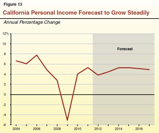
Personal Income in California Projected to Grow Steadily. As shown in Figure 13, we forecast that California personal income (not adjusted for inflation) will increase 3.8 percent in 2012, followed by somewhat stronger growth of 4.5 percent in 2013. Personal income growth is being aided by healthy wage and salary growth in high–income labor markets, especially the technology sector centered in the Silicon Valley. Areas of the state with concentrations of these high–income labor markets likely will continue to outperform most other areas in 2012 and 2013. We project that California personal income will grow at about 5 percent per year from 2014 to 2017, as the housing market and related construction sectors begin to contribute more to the California economy. Our personal income growth estimates for 2012 are somewhat lower than they were in our November forecast due to slower assumed growth in non–wage income sources.
Housing Market and Construction Industry Forecasted to Remain Sluggish. Given the surplus stock of single–family homes and generally weak demand for housing, we expect new single–family housing starts to remain well below their pre–recession levels for the next several years. Construction–related employment in California, accordingly, is forecast to increase only marginally in 2012 before beginning modest growth in 2013 and 2014.
Some Weakening State Revenue Data Has Materialized in Recent Months. Our updated forecast of General Fund revenues and transfers—including the revenue impact of the Governor’s proposed tax initiative—is summarized in Figure 14. While economic forecasts have improved somewhat since our last forecast in November, data received after that forecast concerning 2010 tax payments by Californians, as well as weak PIT estimated payments in December and January, have weakened some parts of our revenue outlook.
Figure 14
LAO February 2012 Revenue Forecasta
General Fund—Assumes Bush Tax Cuts Expire at End of 2012 (In Millions)
|
|
2011–12
|
2012–13
|
2013–14
|
2014–15
|
2015–16
|
2016–17
|
|
Personal income tax
|
$51,405
|
$55,720
|
$55,391
|
$60,080
|
$64,183
|
$66,198
|
|
Sales and use tax
|
18,593
|
21,157
|
24,010
|
25,764
|
27,453
|
27,595
|
|
Corporation tax
|
9,415
|
9,277
|
9,385
|
10,029
|
10,671
|
10,834
|
|
Subtotals, “Big Three” Taxes
|
($79,413)
|
($86,154)
|
($88,786)
|
($95,873)
|
($102,307)
|
($104,627)
|
|
Insurance tax
|
$2,103
|
$2,091
|
$2,262
|
$2,370
|
$2,474
|
$2,572
|
|
Other revenuesb
|
2,700
|
2,750
|
2,200
|
2,300
|
2,400
|
2,500
|
|
Net transfers and loansc
|
1,425
|
850
|
–1,000
|
–500
|
—
|
50
|
|
Total Revenues and Transfers
|
$85,641
|
$91,845
|
$92,248
|
$100,043
|
$107,181
|
$109,749
|
We discussed most of these recent trends in our January report,
Overview of the Governor’s Budget. At that time, we indicated that our November forecast of “baseline” (current–law) General Fund revenues was $4.7 billion lower than the administration’s January forecast for 2011–12 and 2012–13 combined. Moreover, our earlier estimate of the revenue effect of the Governor’s proposed tax initiative was $2.1 billion lower than the administration’s, for a total difference of about $6.8 billion in 2011–12 and 2012–13 combined.
Updated Forecast: $6.5 Billion Lower Than Administration in 2011–12 and 2012–13 Combined. As shown in Figure 15, our new General Fund revenue forecast is $3 billion less than the administration’s in 2011–12 and $3.5 billion less in 2012–13, for a total difference of $6.5 billion across the two fiscal years. As discussed below, this new forecast—unlike prior ones—includes (1) the revenue effects of the Governor’s proposed tax initiative and (2) a rough, initial estimate of PIT revenues the state may receive related to a possible IPO by Facebook, Inc. If the Facebook–related revenues were omitted from this new forecast, General Fund revenues would be about $8.5 billion lower than the administration’s in 2011–12 and 2012–13 combined—weaker than the $6.8 billion difference identified in January—due mainly to the various revenue issues mentioned above that have materialized over the last three months.
Figure 15
LAO Forecasts Lower Revenues Than the Administration
General Fund, Assumes Bush Tax Cuts Expire at End of 2012 (In Millions)
|
|
2011–12
|
|
2012–13
|
|
LAO February Forecasta
|
Governor’s Budget Forecast
|
LAO February Forecasta
|
Governor’s Budget Forecast
|
|
Personal income tax
|
$51,405
|
$54,186
|
|
$55,720
|
$59,552
|
|
Sales and use tax
|
18,593
|
18,777
|
|
21,157
|
20,769
|
|
Corporation tax
|
9,415
|
9,479
|
|
9,277
|
9,342
|
|
Subtotals, “Big Three” taxes
|
($79,413)
|
($82,442)
|
($86,154)
|
($89,663)
|
|
Insurance tax
|
$2,103
|
$2,042
|
|
$2,091
|
$2,179
|
|
Other revenues
|
2,700
|
2,709
|
|
2,750
|
2,706
|
|
Net transfers and loans
|
1,425
|
1,413
|
|
850
|
841
|
|
Total Revenues and Transfers
|
$85,641
|
$88,606
|
$91,845
|
$95,389
|
|
Difference—LAO February Forecast Minus Governor’s Budget
|
–$2,965
|
|
–$3,544
|
Effect on Budget Problem. Lower revenues make it more difficult for the state to balance its budget in any given fiscal year. If our revenue forecast proves to be more accurate than the administration’s, it means that the Legislature and the Governor will have to identify other budgetary solutions to bring the 2012–13 state spending plan into balance. The net effect of our lower revenue assumptions on the near–term budget problem, however, will depend on how the forecast affects the Proposition 98 minimum guarantee for schools and community colleges. We expect to develop updated Proposition 98 estimates in the coming weeks.
Assumptions Concerning Taxpayer Behavior. As discussed in more detail below, our PIT forecast, in particular, reflects various assumptions about federal tax policy and how they might affect taxpayer behavior. The forecast data shown in Figures 14 and 15 adhere to similar basic assumptions as those included in the administration’s January revenue forecast in order to allow for simpler comparisons. Later in this section, we discuss how changes in some of those assumptions could affect the revenue outlook for 2011–12 and beyond.
PIT Forecast Affected by Rate Changes and Facebook. General Fund PIT revenues for 2010–11 are estimated to have totaled $49.5 billion. Midway through 2010–11, temporary legislative measures to increase PIT revenues expired. These temporary measures adopted in 2009 included a 0.25 percentage point increase in each PIT marginal tax rate and a decrease in the value of the state’s dependent credit. The expiration of the temporary measures has reduced the growth of PIT revenues in 2011–12—the first full fiscal year after the expiration of the temporary increases—by a few percentage points compared to what their growth otherwise would have been. Despite this effect, we forecast that growth in the income of California taxpayers will be sufficient to keep PIT collections roughly steady in 2011–12 at $49.4 billion, excluding the effects of the Governor’s proposed tax initiative and the possible Facebook IPO. When those additional effects are included, our base PIT forecast for 2011–12 rises to $51.4 billion, a 3.9 percent increase above 2010–11.
In 2012–13, the first full fiscal year in which the Governor’s proposed tax initiative would affect budget revenues, our base PIT forecast rises to $55.7 billion, up 8.4 percent from 2011–12. About one–fourth of this increase is attributable to there being a full year of PIT revenues in 2012–13 resulting from the Governor’s initiative (as compared to the half year of initiative revenues assumed to be accrued to 2011–12). Another one–fourth of the annual increase is attributable to our assumption concerning Facebook IPO–related tax collections (discussed in more detail below), which the company’s prospectus hints will peak during the 2012–13 fiscal year. Over 4 percentage points of the growth—around one half of the total—is attributable to assumed taxable income increases. These various factors are summarized in the “Base Scenario” section of Figure 16, which makes similar assumptions concerning federal tax policy and accelerations of capital gains and other income as those included in the administration’s January budget estimates. Other scenarios listed in Figure 16 use different assumptions, as discussed below.
Figure 16
Alternate Personal Income Tax (PIT) Forecast Scenarios
General Fund (In Millions)a
|
|
2011–12
|
2012–13
|
2013–14
|
2014–15
|
2015–16
|
2016–17
|
|
Base Scenario—Assume Bush Tax Cuts Expire at End of 2012
|
|
|
|
|
|
Excluding Governor’s Initiative and Facebook
|
$49,377
|
$51,771
|
$52,615
|
$57,069
|
$61,139
|
$64,970
|
|
Governor’s Initiative
|
1,528
|
2,449
|
2,576
|
2,811
|
2,994
|
1,228
|
|
Facebook–Related PIT Revenuesb
|
500
|
1,500
|
200
|
200
|
50
|
—
|
|
Totals, Base Scenario
|
$51,405
|
$55,720
|
$55,391
|
$60,080
|
$64,183
|
$66,198
|
|
Alternate Scenario 1—Assume Bush Tax Cuts Expire at End of 2013
|
|
|
|
|
|
Excluding Governor’s Initiative and Facebook
|
$49,096
|
$52,017
|
$53,553
|
$56,420
|
$60,898
|
$64,953
|
|
Governor’s Initiative
|
1,499
|
2,542
|
2,570
|
2,757
|
2,994
|
1,228
|
|
Facebook–Related PIT Revenuesb
|
500
|
1,500
|
200
|
200
|
50
|
—
|
|
Totals, Alternate Scenario 1
|
$51,095
|
$56,059
|
$56,323
|
$59,377
|
$63,942
|
$66,181
|
|
Alternate Scenario 2—Assume Bush Tax Cuts Are Extended Indefinitely
|
|
|
|
|
|
Excluding Governor’s Initiative and Facebook
|
$49,096
|
$51,694
|
$52,922
|
$57,118
|
$61,145
|
$64,968
|
|
Governor’s Initiative
|
1,499
|
2,458
|
2,595
|
2,811
|
2,994
|
1,228
|
|
Facebook–Related PIT Revenuesb
|
500
|
1,500
|
200
|
200
|
50
|
—
|
|
Totals, Alternate Scenario 2
|
$51,095
|
$55,652
|
$55,717
|
$60,129
|
$64,189
|
$66,196
|
Near–Term Collections May Be Affected by Behavioral Responses to Tax Policy Changes. As discussed earlier in this report, there currently exists a significant amount of uncertainty concerning a variety of elements of future federal tax policy. Tax policy changes may have a significant effect over the next few years on when and how some taxpayers choose to realize stock market and other asset gains and even other kinds of income. In particular, wealthy taxpayers—who pay a significant share of California’s income taxes—have considerable opportunity to accelerate or delay their realization of capital gains, as well as certain other forms of income, in response to tax policy changes. To the extent such taxpayers respond in this manner, the state may collect certain revenues earlier or later than it otherwise would.
For example, in our base forecast scenario, we now assume—like the administration—that the Bush tax cuts expire as required under current federal law at the end of 2012. The Bush tax cuts include reductions of taxes on long–term capital gain and qualified dividend income, as well as other types of income. In addition to the scheduled expiration of the Bush tax cuts, the federal Patient Protection and Affordable Care Act imposes a 3.8 percent Medicare tax on certain categories of unearned income (such as certain investment–related income) for certain high–income taxpayers, which will go into effect on January 1, 2013. This means that under current federal law, taxpayers will pay a higher tax rate on income realized after the beginning of 2013. To the extent that a taxpayer can accelerate 2013 income to 2012, therefore, the taxpayer may be able to pay a lower tax rate. Accordingly, in our base forecast scenario, we assume that about 20 percent of capital gains income; 5 percent of dividend, interest, and rent income; and 1 percent of wages and salaries that otherwise would be realized in 2013 will be accelerated to 2012. This tends to increase certain categories of state revenue collections in 2011–12 and 2012–13, with offsetting reductions in various revenue categories, particularly in 2012–13 and 2013–14. For the most part, these behavioral responses would affect the state’s high–income taxpayers, who pay the highest marginal PIT rates.
Many economists’ revenue forecasts—including both our own and the administration’s January 2012 economic forecast—assume that Congress and the President will agree to various fiscal and tax measures later this year to provide additional support to the fragile economy, including an extension of the Bush tax cuts for at least one year. Figure 16 displays such an alternate scenario (listed as “Alternate Scenario 1”), which assumes that the Bush tax cuts expire instead at the end of 2013. In this scenario, since the Medicare tax takes effect in 2013, we are now assuming that this tax causes taxpayers to accelerate receipts of 15 percent of their 2013 capital gains and 4 percent of their 2013 dividends, interest, and rent from 2013 to 2012. Furthermore, in Alternate Scenario 1, we assume that the expiration of the Bush tax cuts at the end of 2013 causes acceleration of 15 percent of capital gains; 4 percent of dividends, interest, and rent; and 1 percent of wages to be accelerated from 2014 to 2013.
Figure 16 displays another scenario (“Alternate Scenario 2”), in which the Bush tax cuts never expire and there is no behavioral response other than the response related to the Medicare tax described in Alternate Scenario 1. Thus, all three scenarios shown in Figure 16 assume accelerations of 2013 income to 2012. (Our November forecast did not.)
Behavioral responses of the types included in our base forecast and the alternate scenarios are impossible to predict with precision and difficult to evaluate even in retrospect, given tax agencies’ inability to know which capital gains and other income were accelerated and which were not. In fact, many other scenarios are possible. For example, assuming that Congress and the President do not make major decisions on federal tax policy until very late in the year (after the November 2012 election), some taxpayers will accelerate income no matter what final decision is made regarding extension of the Bush tax cuts. In addition, in any of these scenarios, we cannot predict well when taxpayers will begin to make payments to the state, which could affect the fiscal years to which revenue is accrued under existing and proposed revenue accrual policies (discussed later in this report). Moreover, while there may be several tax proposals on the November 2012 statewide ballot, none of our scenarios assume that taxpayer accelerations are increased more due to possible state tax policy changes. All of these challenges in predicting the precise nature and degree of behavioral responses could easily drive PIT revenues higher or lower by hundreds of millions of dollars per year over the next few years.
Capital Gains Income Notoriously Difficult to Forecast. In our January 2012
Overview of the Governor’s Budget, we discussed our concerns that the administration’s current method of forecasting high–income tax filers’ income—especially capital gains—tended to overestimate PIT growth over the next few years, including revenue growth that would result from the Governor’s tax initiative. In a statement released on February 10, DOF noted that one reason for weaker–than–projected estimated payments by PIT taxpayers in December and January could be that 2011 capital gains were lower than assumed in the Governor’s budget. Our updated forecast assumes that this is the case. Moreover, given the assumptions about future stock market and home price growth embedded in our economic forecast (which we believe are similar to the administration’s), we can identify no strong rationale for the administration’s assumption that capital gains will grow very rapidly in 2012 and later years. Our much lower forecast of future capital gains growth—along with key forecast assumptions concerning stock and home prices—is summarized in Figure 17.
Figure 17
Capital Gains Forecasts
Assumes Bush Tax Cuts Expire at End of 2012 (Dollars in Billions)
|
|
LAO February Forecast
|
|
Governor’s Budget Forecast
|
|
Annual Growth of Stock Price Indexa
|
Annual Appreciation of California Home Pricesb
|
California Resident Net Capital Gainsc
|
California Resident Net Capital Gains
|
|
Actual
|
|
|
|
|
|
|
2003
|
–3.2%
|
18.0%
|
$46
|
|
$46
|
|
2004
|
17.3
|
25.9
|
76
|
|
76
|
|
2005
|
6.8
|
21.7
|
112
|
|
112
|
|
2006
|
8.6
|
6.1
|
118
|
|
118
|
|
2007
|
12.7
|
–8.7
|
132
|
|
132
|
|
2008
|
–17.3
|
–26.7
|
56
|
|
56
|
|
2009
|
–22.5
|
–15.9
|
29
|
|
29
|
|
Forecastd
|
|
|
|
|
|
|
2010
|
20.3
|
2.1
|
52
|
|
55
|
|
2011
|
11.4
|
–6.5
|
54
|
|
63
|
|
2012
|
6.8
|
–3.7
|
70
|
|
96
|
|
2013
|
5.4
|
2.5
|
50
|
|
69
|
|
2014
|
5.4
|
3.0
|
69
|
|
93
|
|
2015
|
5.5
|
3.1
|
76
|
|
101
|
|
2016
|
5.9
|
3.1
|
83
|
|
NA
|
|
2017
|
5.2
|
3.1
|
90
|
|
NA
|
The level of net capital gains realized by California taxpayers each year is dependent on a complex variety of factors, including recent growth of asset prices (such as stock, bond, or home prices) and the “carryover effect” of prior–year declines in asset prices. In recent years, as shown in Figure 17, both house and stock prices declined significantly, which resulted not only in near–term reductions in net capital gains but also reductions in the value of assets destined to be sold in the future for either a capital gain or loss. Taking all of these effects together, our revenue forecasting models show that net capital gains have increased during periods of sustained growth in asset markets (2004 through 2007, for instance), decreased during periods of asset market declines (2008 and 2009), and increase thereafter, but from a lower base level (as shown in 2010). Our 2010 capital gains forecast generally reflects preliminary Franchise Tax Board data, which showed that despite the significant stock market gains of that year, the level of capital gains was significantly depressed from its pre–recession bubble levels and about $14 billion lower than assumed in our November forecast.
In 2011, stock market gains were less notable than they were in 2010, and these gains were unevenly distributed throughout the calendar year, as markets climbed for much of the first half of the year (far above their levels from early 2010) and then sharply decreased in the summer and fall before climbing again late in the year. Thus, while the S&P 500 index, on average, was about 11 percent higher during 2011 than in 2010, an individual investor might have sold a security for significant gains at one point in the year but for little or no gain (or even a loss) at some other point in 2011. Overall, our forecasting model suggests these trends will lead to a small increase in California capital gains in 2011. In 2012, our base capital gains forecast is elevated by the accelerations related to federal tax policy, as discussed earlier.
In general, assuming steady, moderate upward growth in stock and home prices, we believe capital gains will tend to climb a few percent per year in the future. Strong stock and housing market years could produce some of the very strong capital gains reflected in the administration’s forecast. In our view, however, the economic conditions supporting such an outcome are not yet in evidence.
High–Income Taxpayers’ Wage and Other Income Continues to Increase. In our May 2011 publication, The 2011–12 Budget: Overview of the May Revision, we discussed differences between our forecast and the administration’s forecast concerning wage and salary growth for both upper–income taxpayers and other taxpayers. Differing assumptions on wage levels and growth for 2010 and later years have marked recent forecasts. These assumptions are important to PIT forecasts, given the state’s reliance on tax payments by higher–income individuals. Developing these wage forecasts recently has been very challenging since both our office and the administration have to estimate how taxpayer income will recover from the recent, unprecedented recession, and hard data on these topics from FTB is not received until well after the year in question has ended.
Since last May, differences between our two forecasts have narrowed, as the administration has increased its estimates of 2010 wage and salary growth for taxpayers with under $200,000 of adjusted gross income (AGI) and decreased its estimates for wage growth of taxpayers with over $200,000 of AGI. At the same time, based on the data available to us, our office has increased our estimate of 2010 wage growth for upper–income taxpayers and decreased slightly our wage growth assumptions for lower–income taxpayers. Our current forecasts’ assumptions concerning wage growth are summarized in Figure 18.
Figure 18
Wage Forecast Comparisons
Percent Growth in Wages and Salaries Over Prior Year
|
|
LAO February Forecast
|
|
Governor’s Budget Forecast
|
|
Total Wages
|
Wages for Filers Under $200,000 AGI
|
Wages for Filers Over $200,000 AGI
|
Total Wages
|
Wages for Filers Under $200,000 AGI
|
Wages for Filers Over $200,000 AGI
|
|
2010
|
3.8%
|
0.4%
|
15.5%
|
|
2.1%
|
–0.8%
|
11.8%
|
|
2011
|
4.6
|
3.9
|
6.9
|
|
4.8
|
3.5
|
8.7
|
|
2012
|
5.7
|
5.0
|
8.0
|
|
4.9
|
3.9
|
7.5
|
|
2013
|
2.8
|
1.8
|
5.5
|
|
2.3
|
1.8
|
3.6
|
Since our November forecast, we have increased our wage forecasts somewhat, and we have also increased substantially our forecasts for annuity income (which is received by lower–income and middle–income tax filers, in particular). Other income forecasts have been adjusted downward based largely on data received from FTB after our November forecast, especially dividends, interest, and rent income (received primarily by higher–income filers). On net, we now generally assume higher taxable incomes than we did in November for California tax filers with $5 million and over in annual income, higher income in some forecast years for filers with $1 million to $5 million in income, and somewhat lower income in some years for filers with $500,000 to $1 million in income. These changes in assumptions affect not only our forecast of current–law PIT revenues, but also our forecast of PIT revenues that would be generated by the Governor’s initiative (now up by a few hundred million dollars in some years, compared to our prior estimates).
Our income distribution model discussed above does not consider the effects of the possible Facebook IPO, which could generate extraordinary, one–time changes in high–income taxpayer data in 2012 and 2013.
Facebook’s IPO, if It Occurs, Would Help State Revenues. In this forecast, we make an initial—and very rough—effort to incorporate PIT revenues the state would receive due to the possible Facebook IPO, which is widely expected to occur later this spring with an initial market capitalization (the overall value of the business in the stock market) of around $100 billion. Facebook’s Form S–1, its preliminary prospectus in advance of the possible IPO, contains hints about future anticipated tax liabilities of both Facebook investors and employees and the company itself. In particular, the prospectus discusses in varying levels of detail the IPO–related tax liabilities of (1) Facebook employees and others with option–like assets known as “restricted stock units” and (2) the company’s founder and chief executive officer, Mark Zuckerberg. While the prospectus contains important information in this regard, it lacks many details, some of which will be clarified in the days prior to the IPO and some of which will not. For example, the prospectus does not contain certain detailed information on several types of compensation provided to Facebook employees and executives, such as a description of the full variety of instances in which those persons could delay receipt of such compensation to later dates. Importantly, the prospectus also does not describe in detail the precise manner in which various stock–related transactions with executives, employees, and others will result in withholding obligations to federal and state tax agencies. The prospectus also cannot tell us which of the company’s current major investors are Californians and when they may be motivated to sell their Facebook shares. Perhaps most significantly, the preliminary prospectus does not tell us when the IPO will occur and at what stock price, which will affect when (and in what fiscal years) tax revenues materialize and in what dollar amounts.
Given all of these uncertainties, there is a very large range of error around our initial Facebook PIT estimates, which are shown in Figure 16. Specifically, we are assuming in our forecast receipt of $500 million of PIT revenue in 2011–12 (assuming an IPO prior to the end of the current fiscal year results in significant PIT withholding or estimated payments in 2011–12), $1.5 billion in 2012–13, and much smaller amounts thereafter through 2015–16. Should the IPO proceed, it appears virtually certain that the state revenue impact will be at least in the hundreds of millions of dollars, spread across a few fiscal years. On the other hand, if the IPO results in a market capitalization of well over $100 billion and/or Facebook’s stock price climbs significantly above its IPO level (particularly in the first 6 to 12 months after the IPO), the state revenue benefit could be $1 billion or more over the level we assume, spread across a few fiscal years. At this time, based on the limited information available to us, we believe the numbers included in our forecast are a reasonable initial estimate. As we discussed in the Overview of the Governor’s Budget, the Facebook impact on state revenues cannot be predicted in advance and will never be known retrospectively with any degree of precision. Yet, given that an IPO clearly would benefit state revenues, we believe it is appropriate for policymakers to incorporate this into their budgetary discussions—whether they decide to expend Facebook–related PIT revenues in advance of their receipt or, alternatively, to adopt a more cautious approach in light of the many uncertainties in this area.
Revenue Accrual Policies Increasingly Challenging to Model. We last discussed the state’s approach to accruing (attributing) PIT and other revenues to particular fiscal years in our 2011 report, The 2011–12 Budget: The Administration’s Revenue Accrual Approach. The Legislature rejected the administration’s accrual modification proposal in 2011, but the administration now proposes to accrue a small portion of PIT revenue—principally that related to the Governor’s initiative—under a similar method as that proposed last year. In our forecasting models, we attempt to apply the administration’s revenue accrual practices, but we acknowledge that our ability to do so accurately is limited for a variety of reasons, including recently adopted tax policy provisions that have changed markedly the dates when some tax payments are received, which in turn can affect when revenues are accrued. The various uncertainties in the accrual policies and the resulting forecast difficulties mean that our projections easily can be hundreds of millions of dollars too high or too low in any given fiscal year due to accrual and payment date issues. We suspect that these uncertainties will persist for a while, until at least several years have passed without significant PIT timing, accrual, or other major tax policy changes.
We continue to observe, as we did last year, that the state’s current and proposed revenue accrual practices make it more difficult to accurately estimate revenues, risk inconsistency among the state departments that develop and audit financial records, and promote confusion for bond investors who use the state’s financial statements. In some years, the state’s overall accrual practices may allow it to spend more than it can afford and in other years may result in lower Proposition 98 spending requirements than otherwise would be the case. The inconsistencies embedded in the state’s budgetary revenue and expenditure accounting have multiplied in recent years, which we find to be a troubling trend. The administration’s proposed changes to accruals have some merit, as we noted last year, but over the longer term, the state should move in a direction of adhering to consistent, appropriate, and publicly transparent accrual methods for all sources of revenue.
We estimate that General Fund sales and use tax (SUT) revenues will total $18.6 billion in 2011–12. In 2012–13, assuming passage of the Governor’s proposed tax initiative, we estimate that General Fund SUT revenues will increase to $21.2 billion, a 13.8 percent increase from 2011–12. Approximately half of this increase is due to the Governor’s initiative proposal, which would increase the General Fund portion of the SUT rate by 0.5 percentage points (from 3.9375 percent to 4.4375 percent) for four calendar years—from January 1, 2013 through December 31, 2016. The other half is the result of underlying growth in the SUT base of 7 percent. The SUT revenues follow a similar trend in 2013–14—the first full–year effect of the Governor’s initiative proposal—increasing 13.5 percent to $24 billion.
Taxable Sales Fell Disproportionately During the Recession. The main determinant of SUT revenues is taxable sales. California taxes sales and use of most tangible products but excludes virtually all services. About two–thirds of taxable sales result from retail spending by consumers, including a significant portion on vehicles and large household purchases, both of which declined sharply during the recession. Other important categories of taxable sales are the purchase of building materials involved in new construction and business–to–business taxable transactions, where the purchasing business is the final consumer of the sold item.
Between the second quarter of 2008 and the second quarter of 2009, taxable sales declined by 17 percent while personal income fell by just 6 percent. The reduction in taxable sales relative to income—illustrated in Figure 19—was the result of: (1) consumers and businesses curtailing costly purchases such as household appliances, new vehicles, and business machinery; (2) increased household savings rates; and (3) the long–term trend toward greater consumption of nontaxable goods (services and other products, such as those purchased online, for which the collection of SUT is limited) as a fraction of total consumption.
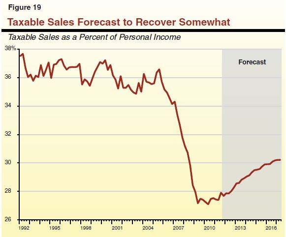
Taxable Sales Now Making Up Lost Ground. Since the start of the recovery, taxable sales have rebounded faster than personal income, signaling a correction to the decline in taxable sales discussed above. Thus, in Figure 19, taxable sales as a percent of personal income has been growing since 2010. We expect this trend to continue throughout the forecast period, as consumers and businesses gradually return to more normal levels of taxable spending relative to income.
Risks and Uncertainties in the SUT Forecast. Taxable sales are heavily influenced by (1) employment and income growth, (2) household savings rates, (3) the availability of consumer and business credit, and (4) overall confidence in the economy. These factors could differ from our forecast in several ways.
- Incomes, Employment, and Prices Affect Consumption. We project that personal income and employment in California will increase modestly throughout 2012 and 2013. Should actual incomes grow faster, or slower, than we project, SUT revenues could vary significantly from our forecast. Other factors, such as gasoline and grocery prices—even though the state does not collect General Fund sales taxes on these items—could influence taxable sales as well. This is because consumers may reduce spending on taxable items in order to pay higher prices of other goods such as these.
- Household Savings Rates Influence Spending Decisions. In recent months, national household savings rates have fallen to pre–recession levels, likely indicating that savings built up over the past few years have supported some recent growth in taxable sales. Should this decline indicate that consumers are becoming more confident about their personal finances, taxable sales could be somewhat higher than we project. If, on the other hand, lower savings rates are more the result of households’ difficult financial circumstances, stagnant wages, and stubbornly high unemployment, consumers may end up curbing spending on taxable items more than reflected in our projections.
- Consumer and Business Credit Availability Influences Spending Decisions. In recent months credit availability has improved somewhat, although lending standards remain relatively tight compared to pre–recession levels. Households tend to use credit to finance large taxable purchases—such as vehicles, appliances, personal electronics, and home improvements—and business credit allows firms to make fixed investments in equipment, computer systems, and buildings that often are too costly to finance in any single year. Our forecast assumes that this trend toward more expansive credit continues in future years.
- Consumer Confidence About the Economy May Affect Future Spending. Taxable sales in California sustained a pronounced recovery through the summer months—increasing at an annual rate of 9 percent during the second quarter and 8 percent during the third quarter—despite the fact that the economy slowed considerably and consumer sentiment fell to recession–levels. As the economy has improved in recent months, so has consumer sentiment (also known as consumer confidence). Consumer confidence now appears to be a significant factor in recent taxable sales growth. Our economic forecast makes assumptions about consumer confidence trends, as measured by the Reuters/University of Michigan Consumer Sentiment Index. In general, we assume that consumer confidence continues to climb through 2013 and then generally stabilizes for the remainder of our forecast period.
Policy Changes That Occurred in 2010 Have Reduced General Fund SUT Receipts. In 2011–12, General Fund SUT receipts will decline significantly from 2010–11 levels, reflecting the net effect of: (1) the “fuel tax swap” passed by the Legislature in 2010, under which the state no longer collects sales tax on gasoline, (2) the shift of some state responsibilities to local government—known as “realignment”—which redirects over $5 billion in SUT receipts to cities and counties (see box below), (3) the expiration of the temporary 1 percent SUT rate increase adopted in 2009, and (4) projected growth in the SUT tax base of 6.6 percent. Policy changes and underlying growth, taken together, reduce state General Fund SUT revenue from $27 billion in 2010–11 to a projected $18.6 billion in 2011–12.
|
As part of the 2011–12 budget plan, the Legislature enacted a major shift—or “realignment”—of state program responsibilities and dedicated revenues to local governments. The realignment package allocates state sales and use tax (SUT) and vehicle license fee (VLF) revenues to local governments—primarily counties—in order to fund certain public safety and health and human services programs. Specifically, on an ongoing basis, realignment allocated revenues from 1.0625 percentage points of the existing SUT rate that previously went to the General Fund to local governments, as well as certain VLF revenues. Our updated projections for these revenue sources are shown in the figure below.
2011 Realignment Revenues
(In Millions)
|
|
2011–12
|
2012–13
|
2013–14
|
2014–15
|
2015–16
|
2016–17
|
|
Sales and use tax
|
$5,107
|
$5,488
|
$5,880
|
$6,302
|
$6,709
|
$7,118
|
|
Vehicle license fee (VLF)a
|
462
|
496
|
492
|
492
|
492
|
492
|
|
Totals
|
$5,569
|
$5,984
|
$6,372
|
$6,794
|
|
$7,610
|
|
Despite Higher Profits, Corporation Tax Likely to Decline Through 2012–13. Corporation tax (CT) revenues for 2010–11 are estimated to have totaled $9.6 billion. As we have discussed in recent publications, the Legislature made several significant changes to CT policies in recent years, several of which were intended to accelerate CT collections. Such actions helped the state balance its General Fund budget over the last few years but are now beginning to have a negative impact on the state budgetary situation, as we discuss below. In large part due to the lingering effects of these policy changes, we project that the state’s CT revenues will be slightly lower in 2011–12 and 2012–13—$9.4 billion and $9.3 billion, respectively—before growing to reach $10.8 billion in 2016–17. Under our projections, CT revenue would remain below the pre–recession high ($11.8 billion in 2007–08) through at least 2016–17.
Recent CT Policy Changes Now Resulting in Lower State Revenues. Despite significant growth in corporate profits, tax revenues have fallen due largely to significant tax policy changes of recent years. It is difficult to isolate the revenue impacts of these changes from other factors affecting revenues. That said, our best estimate is that in 2007–08, 2008–09, and 2009–10, policy changes had the net impact of increasing CT revenues, as shown in Figure 20. This was intentional, as the state implemented policies that accelerated CT collections from future years in order to help cope with budgetary challenges resulting from the recession. These actions include the suspension, for 2008 through 2011, of larger businesses’ use of net operating loss deductions. In addition, penalties on corporate taxpayers who are found to have significantly underpaid their taxes also serve to accelerate CT collections. This occurs as businesses try to avoid penalties by paying up front some of the tax they might have paid later following an audit.
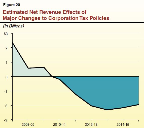
In addition to the revenue accelerations, Figure 20 also includes the effects of recent policy changes that reduced CT revenues, rather than just accelerating their collection. The most significant of these is the elective single sales factor—the new option for multistate businesses to choose each year which method they use to determine their California taxable income. This provision is estimated to reduce CT revenues by around $1 billion per year. Under another major policy change, tax credits are now easier to use due to a law that allows transfers of certain credits between companies that are treated as parts of a single business group for tax purposes.
By 2011–12, the expected net effect of the recent CT policy changes (including both revenue accelerations and tax reductions) has been to lower revenues by around $1.2 billion, compared to estimates of what revenues would have been without these major tax policy changes. This net negative effect is expected to grow to around $2 billion annually for the remainder of our forecast period. Due in part to the recent changes, our model now suggests that corporations pay an effective state tax rate of around 5 percent. (This is the percentage of corporate profits actually paid in taxes, after considering all credits, deductions, and other factors that reduce tax payments below the statutory rates.)
New Information Drives Changes Since Our Last Forecast. Our updated CT projections are somewhat lower than those in our November 2011 CT forecast—by over $150 million in 2012–13 and several hundred million dollars per year thereafter. These changes are the net result of new and revised data in two main areas: corporate profits and tax credit usage.
First, corporate profits taxable by California—the main driver of our CT revenue forecast—now are projected to be slightly higher through 2013 than we previously projected and slightly lower in 2014 and beyond. This is shown in Figure 21.
A more significant factor in driving forecast CT revenues downward since November is updated data concerning usage of the state’s largest CT credit, the research and development (R&D) credit. A major surprise in taxpayer data from the 2010 tax year—which was not available when we prepared our November 2011 forecast—was the degree to which the rebound in corporate profits was offset by greater use of tax credits, especially the R&D credit. Figure 22 shows the sharp increase in R&D credit usage in 2010. This change has led us to increase our estimates of R&D credit usage for future years as well. On its own, this revision reduces 2011–12 revenues by roughly $600 million and later years’ revenues by roughly $300 million per year.
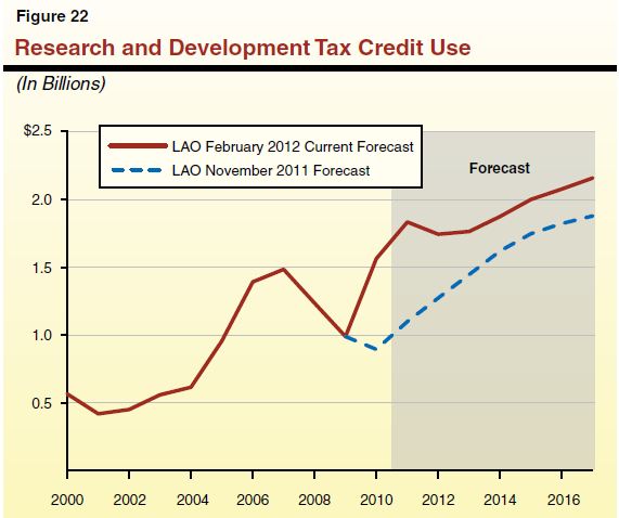
Tax credit use is hard to predict in part because the link between credit use and profits is complex. Profits drive pre–credit tax liabilities, and when pre–credit tax liabilities increase, tax credit use essentially increases dollar for dollar in the group of taxpayers that have enough accumulated credits to minimize their tax liabilities. In contrast, for the group of taxpayers that do not have as many accumulated credits, use of credits can increase by less than pre–credit tax liabilities do. While we observe and forecast changes in aggregate corporate profits, it is impossible to predict with precision how increased profits will be distributed to the groups of companies with the two profiles described above.
There is a significant likelihood that future years’ tax data will reveal even more surprises about use of the R&D and other CT credits and deductions. For example, recent legislation allowing transfers of certain tax credits between business entities within a single family of companies will introduce more uncertainty into future CT forecasting. To a large extent, how this and other policy changes will affect CT revenues will not be known until companies file future tax returns.
Economic data currently is providing plenty of mixed signals to California’s policymakers, as they continue to craft state and local budgets in a constrained fiscal environment. California’s economy now is clearly improving in many important ways, including employment growth. Nevertheless, significant impediments block the state’s path to a more robust recovery from the recent, staggering economic downturn.
Like the economic data, reports concerning state revenues also have been delivering some mixed messages recently, with recent weakness in income tax payments accompanied by speculation concerning a future bonanza of tax revenues due to the possible Facebook IPO.
If our revenue forecast proves to be more accurate than the administration’s, the Legislature and the Governor will have to identify additional budgetary solutions to bring the 2012–13 state spending plan into balance. Much more information will become available by the end of April, when a large amount of income tax payments are received by the state and refund payments are made. The Legislature will want to wait until after this data is analyzed in the May Revision process before making its 2012–13 budget decisions. We hope that the information provided in this update will help set the stage for the work of legislative budget subcommittees in addressing the state’s fiscal situation.