Projected to End With a Small Reserve. The 2013–14 budget assumed that 2012–13 would end with a $254 million reserve. Our General Fund revenue forecast for 2012–13 now projects $1.65 billion in higher revenues for 2012–13, compared to the budget act’s assumptions. Revenues for 2012–13 ended stronger than was assumed, principally due to personal income tax (PIT) collections. Our higher revenue forecast results in $1.75 billion in additional General Fund expenditures under the Proposition 98 minimum guarantee. That is, for every $1.00 of extra revenue, state spending for schools and community colleges on average is projected to grow by $1.07. This is due to the manner in which the budget plan makes so called “maintenance factor payments” to schools and community colleges. Assuming only minor changes in the entering fund balance, we estimate that 2012–13 ended with a $234 million reserve. While this small reserve equals only 0.2 percent of 2012–13 spending, it nevertheless would be the first positive year–end reserve since 2007–08.
The 2013–14 budget assumed the state would end the fiscal year with a reserve of $1.1 billion. We now estimate that the reserve will more than double—to $2.4 billion—primarily as the net result of the following factors:
- $4.7 Billion in Higher Revenues. Largely due to a higher forecast of capital gains and stronger–than–expected stock price growth, our forecast of PIT revenues for 2013–14 is about $5.2 billion higher than was assumed in the 2013–14 budget. That increase in revenues is partially offset by lower projections of sales and use tax (SUT) and corporation tax (CT) revenues of about $200 million for each of these two tax sources.
- $3.1 Billion in Higher General Fund Proposition 98 Spending. Most of the increased spending in our forecast for 2013–14 is for schools and community colleges. Specifically, we estimate that the Proposition 98 General Fund spending will be $3.1 billion higher than the amount provided in the budget due to our forecast of higher state revenues.
- $0.3 Billion in Other Spending. We estimate that other General Fund spending will be nearly $300 million higher than assumed in the 2013–14 budget. For example, in September 2013 the Legislature passed Chapter 310, Statutes of 2013 (SB 105, Steinberg), which appropriated additional funding to address a federal court order requiring the state to reduce the prison population. We estimate that the California Department of Corrections and Rehabilitation will have net additional spending of nearly $250 million in 2013–14.
These changes have the effect of increasing the 2013–14 operating surplus from the $817 million assumed in the budget to $2.2 billion.
Basis for Our Projections
Purpose of Our Forecast. This forecast does not attempt to predict the budgetary decisions that will be made by the state’s elected leaders. Rather, it is our office’s best estimate of the state’s fiscal condition if current law and current policies remain unchanged through 2019–20. In the near term, therefore, the purpose of this forecast is to provide the Legislature with our best estimate of the resources that will be available in next year’s budget deliberations. Beyond 2014–15, the forecast aims to provide lawmakers with a general sense of the future health of the General Fund budget.
Uses Standard Economic Forecasting Practices. Economic conditions affect not only tax revenues that the state collects, but also state spending levels. For example, the state’s Proposition 98 minimum guarantee for schools and community colleges is determined based on changes in state revenues and economic factors. Further, state spending for health and human services tends to change along with factors such as unemployment, age, and income. Consistent with other mainstream economic forecasts, our forecast assumes that the economy will grow throughout the forecast period. We do not presume that we can predict the timing of recessions.
Forecast Generally Based on Current Laws. Our estimates generally are based on current laws, including those in the State Constitution (such as the Proposition 98 minimum guarantee for schools and community colleges), state statutes, and federal law. In general, this means that we assume taxes and programs operate throughout the forecast period consistent with current law. For example, if state law authorizes a certain tax or program through only part of our forecast period, we generally assume that the law is allowed to play out and that the tax or program expires. For instance, our forecast assumes that the temporary taxes approved by voters in Proposition 30 will expire during the forecast period because it would take a future action either by the Legislature or by voters to extend those taxes.
Forecast Also Considers Certain Recent State Practices. In some cases, we have relied on what has been recent state practice in forecasting revenues and spending. For example, although the state’s hospital quality assurance fee—which offsets General Fund Medi–Cal costs—expires in 2016, the Legislature has extended the fee three times since its initial adoption. In this case, we assume that the current state practice is to continue reauthorizing that fee. Similarly, transfers to the Budget Stabilization Account, the state’s rainy–day fund created by Proposition 58 (2004), have been suspended each year since 2008–09. We assume those suspensions continue throughout the forecast period. Later in this chapter, we discuss how the state might build a comparable reserve under an alternate scenario.
COLAs and Inflation Adjustments Generally Omitted. Consistent with the state laws adopted in 2009 that eliminated automatic cost–of–living adjustments (COLAs) and price increases for most state programs, our forecast generally omits such inflation–related cost increases. This means, for example, that budgets for the universities have not been adjusted for general price increases throughout the forecast period. We include inflation–related cost increases when they are required under federal or state law, as is common in health programs.
Many State Liabilities Remain Unpaid Under Current Law. In the case of state liabilities with repayment dates in state law, we generally assume those liabilities to be repaid according to schedule. For example, our forecast assumes that the deficit–financing bonds authorized by Proposition 57 (2004) continue to be repaid under their established financing mechanism. Other liabilities, however, are not required to be repaid by the state General Fund on any specific timeline under today’s laws and policies. These include some of the items on the Governor’s “wall of debt” (a collection of various budgetary liabilities), along with unfunded liabilities of the California State Teachers’ Retirement System. If the state were to make additional payments toward repaying these liabilities, the operating surpluses projected in our forecast would be reduced by like amounts.
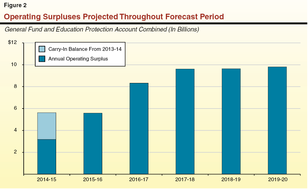
We project that the General Fund operating surplus in 2014–15 will be $3.2 billion, an increase of about $1 billion from our forecast of the 2013–14 operating surplus. Generally, the larger operating surplus is the result of our forecast of revenues growing faster than our forecast of expenditures. In 2014–15, we project that General Fund revenues and transfers will grow 5.7 percent and that spending will grow 4.8 percent. Specifically, our forecast reflects the following:
- $5.8 Billion in Higher Revenues. While revenue growth is expected to be somewhat depressed in 2013–14—due mainly to higher income taxpayers accelerating 2013 income into 2012—we expect revenues to bounce back in 2014–15, principally related to PIT growth. Specifically, we forecast PIT growth in 2014–15 to be 8.1 percent for a year–over–year increase of $5.4 billion. Further, we forecast 2014–15 growth in the CT and SUT to be 6.9 percent and 3.3 percent, respectively.
- $3.3 Billion in Higher General Fund Proposition 98 Spending. Our forecast of healthy revenue growth in 2014–15 produces additional growth in Proposition 98 spending. We estimate that General Fund spending needed to satisfy the Proposition 98 guarantee will increase $3.3 billion over our revised projection of 2013–14 spending levels.
- $1.5 Billion in Higher Spending in Other Parts of the Budget. Outside of Proposition 98, we forecast that spending will increase by $1.5 billion in 2014–15. Most notably, this includes increases of $630 million in debt service on infrastructure bonds and about $600 million in health and human services (excluding California Work Opportunity and Responsibility to Kids [CalWORKs]). The higher spending is offset by increased savings of $650 million related to a decision in the 2013–14 budget to redirect certain realignment funds to help pay for what otherwise would be state costs for CalWORKs.
As shown in Figure 2, we project that operating surpluses will grow at a rate of between about $1 billion and $3 billion each year between 2014–15 and 2017–18, at which point we estimate that they will reach $9.6 billion under current laws and policies. As the temporary taxes authorized by Proposition 30 phase out over several fiscal years near the end of our forecast period, we project that operating surpluses will remain stable as revenues and expenditures grow at similar rates. All this is premised upon our assumption of continuing economic growth through 2020.
In the Near and Medium Term, Strong Revenue Growth. Proposition 30 increased PIT rates on high–income taxpayers from 2012 through 2018, and SUT rates from 2013 through 2016. Under our forecast, Proposition 30 greatly influences revenue growth, particularly in the case of the PIT. Because taxable income has been growing faster for high–income taxpayers, by increasing the marginal PIT rates on those individuals, Proposition 30 has the effect of boosting PIT growth higher than it would be otherwise. In 2014–15 and 2015–16, we forecast total General Fund revenues and transfers to grow 5.7 percent in each year. We project revenue growth to slow thereafter to 4.6 percent in 2016–17 and 4.3 percent in 2017–18, due largely to the phase out of the ¼–cent sales tax increase authorized by Proposition 30.
As Proposition 30 PIT Increases Phase Out—Much Slower Revenue Growth Forecasted. Under Proposition 30, the increase in PIT rates for high–income taxpayers generates a much greater proportion of revenue than the sales tax increase. As a result, the phase out of the higher rates in 2018–19 and 2019–20 has a much more significant impact on revenue growth. Over these two fiscal years, we project that General Fund revenues grow at an average annual rate of only 1.9 percent. As shown in Figure 2, this has the effect of stabilizing the projected trend of annual operating surpluses, as revenues and expenditures grow at similar rates in those two years. In fact, the phase out of Proposition 30 would have had the effect of reducing those operating surpluses in 2018–19 and 2019–20, were it not for projected property tax growth and the end of the “triple flip,” as described below.
General Fund Benefits From Property Taxes, End of Triple Flip in Our Forecast. The Proposition 98 minimum guarantee is funded by two revenue streams—state General Fund support and local property tax revenue distributed to schools. In most years, this local property tax revenue offsets the amount that the state must spend on schools and community colleges, resulting in dollar–for–dollar savings for the General Fund. We project that in the later years of our forecast increases in the Proposition 98 minimum guarantee will largely be paid from school property tax growth. Specifically, while we project that General Fund Proposition 98 spending will increase by 7.8 percent in 2014–15 and 4.4 percent in 2015–16, we forecast it to slow thereafter to an average annual rate of just 0.9 percent for the remainder of the forecast period. The property tax–related factors include:
- Healthy Local Property Tax Growth. As described in Chapter 3, over the next several years, we project underlying local property taxes to grow, on average, about 7 percent each year. This is consistent with average historical growth, but above levels seen in recent years.
- Increased Property Taxes Due to Redevelopment Dissolution. We project that school property taxes related to the dissolution of redevelopment agencies (RDA) will increase from $763 million in 2013–14 to $1.9 billion in 2019–20. These state savings will be offset somewhat by decreases in the revenues from RDA assets over the period.
- End of Triple Flip. Finally, we project that the triple flip—a complex financing mechanism created to repay the state’s deficit–financing bonds of the 2000s—will turn off in 2016–17, resulting in an annual General Fund benefit of about $1.6 billion beginning in 2016–17.
Forecast Reflects Continued Improvement in State’s Finances. In our November 2012 Fiscal Outlook report, we projected that with continued growth in the economy and restraint in new program commitments, the state budget could experience multibillion–dollar operating surpluses within a few years. Since that time, our forecast of General Fund revenues and transfers has increased by a few billion dollars for 2013–14 and 2014–15, and by between $2 billion and $3 billion for each of 2015–16 through 2017–18. In the June budget package for 2013–14, the Legislature and the Governor limited new commitments to a small handful of areas. These factors produce a budgetary situation for 2014–15 that is even more promising than we projected last year.
Surpluses Dependent on Several Key Assumptions. Despite the large reserve that we are projecting for the 2014–15 budget process, the state’s continued fiscal recovery is dependent on a number of assumptions that may not come to pass. Specifically, our forecast assumes:
- Continued Economic Growth. Our forecast assumes steady, moderate economic growth, typical of that seen during a mature economic expansion. This growth drives the increase in revenues and contributes to lower General Fund spending in some areas of the budget (such as CalWORKs grant payments). This assumed economic growth also informs our forecast of local property tax growth, which as mentioned earlier offsets General Fund spending required to meet the Proposition 98 minimum guarantee. Economic growth, therefore, is probably the most important assumption in our forecast.
- Many Budgetary and Retirement Liabilities Remain Unpaid. As described earlier, our forecast assumes that some of the state’s budgetary and retirement liabilities are repaid. For example, we assume that the state increases payments to the California Public Employees’ Retirement System (CalPERS) as required by the CalPERS board, which will reduce the state’s unfunded liabilities for state employee pension benefits over time. Other liabilities, however, are not required to be repaid from the state General Fund on specific timelines under today’s laws and policies. These include some of the items on the Governor’s wall of debt, along with massive retirement liabilities related to the California State Teachers’ Retirement System. If additional payments are made in the future to repay these various liabilities, the operating surpluses in our forecast would be reduced by a like amount. (Besides support from the General Fund, other sources of funding—from school districts and teachers, for example—and other policy decisions may be needed to address some of these liabilities over time.)
Recession Possible During Forecast Period. Like other economic forecasters, we are unable to predict the timing of either a major slowdown in the economy or an actual recession. The severity of the most recent recession may result in a longer–than–average economic expansion. However, it is possible that a recession will occur before 2020. In fact, the current U.S. economic expansion is already over four years old. Since World War II, the average expansion has been just under five years.
Sketch of Hypothetical Recession. To demonstrate the budgetary effects of a possible recession, we have produced one hypothetical recession scenario, as displayed in Figure 3. We developed this scenario to simulate how a moderate recession could affect state finances, but this is merely an illustration of one possible scenario—the severity of an actual recession sometime during the future could be stronger or weaker than that portrayed in Figure 3. In the scenario displayed in Figure 3, revenues fall 10 percent below what our forecast would otherwise be for 2015–16, and then 15 percent below forecasted levels for 2016–17. The revenue losses would be offset somewhat by lower Proposition 98 minimum requirements, and we assume that the state would reduce spending to the lower allowed spending levels. Specifically, the Proposition 98 minimum guarantee would decline 8 percent below what our forecast would otherwise be in 2015–16, and then 12 percent below for 2016–17.
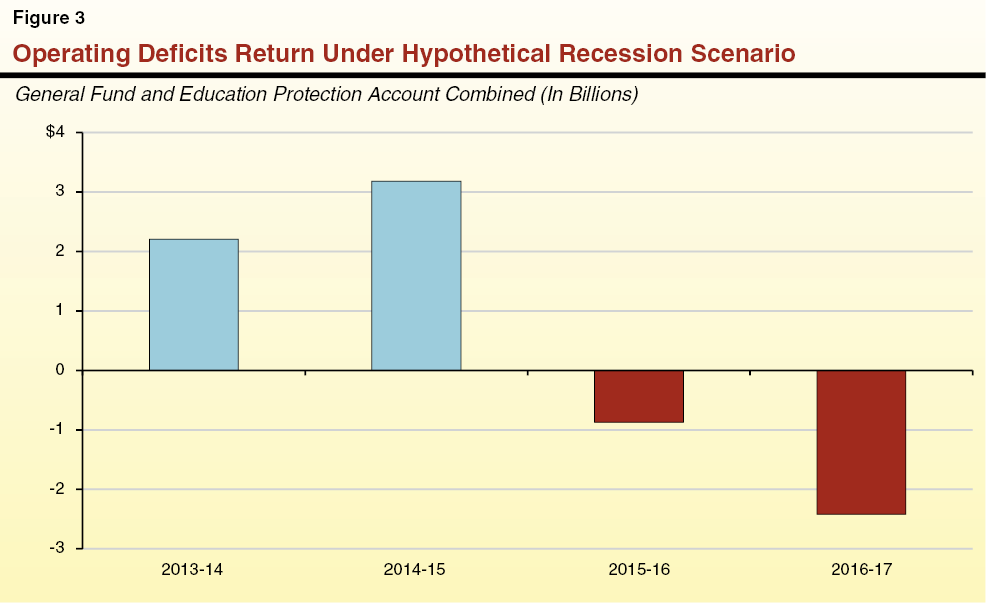
Hypothetical Moderate Recession Would Produce Operating Deficits. In 2013–14 and 2014–15, Figure 3 starts with the same $2.4 billion “carry–in balance” from 2013–14 and the same $3.2 billion operating surplus for 2014–15 as under our standard forecast. Aside from the factors mentioned above, we assume the same set of current laws and policies as under our standard forecast. As such, we assume that no additional ongoing commitments are made in either 2013–14 or 2014–15 and that the entire $5.6 billion is effectively held in reserve. Under this scenario, the state would face a roughly $900 million operating deficit in 2015–16, which would then grow to about $2.4 billion in 2016–17.
A $5.6 Billion Reserve Could Absorb Deficits Under Hypothetical Scenario. As we mentioned earlier, this is merely a sketch of one hypothetical recession. The severity of an actual recession during our forecast period could be stronger or weaker. Nevertheless, absent additional ongoing commitments, the $5.6 billion reserve that we project for the state budget by the end of 2014–15 could more than absorb the combined $3.3 billion in operating deficits over the two–year period of this hypothetical recession. On the other hand, if the entire $5.6 billion were committed to ongoing spending prior to 2015–16, under this scenario the operating deficits would grow by a similar amount (to perhaps $6.5 billion in 2015–16 and $8 billion in 2016–17), requiring the Legislature and the Governor to address large budget shortfalls. This illustration demonstrates the importance of building a sizable reserve in preparation for the next economic downturn. Caution, therefore, is appropriate in weighing new spending both within Proposition 98—as total funding for schools and community colleges would decline under this scenario—and on the non–Proposition 98 side of the budget. Absent a prudent reserve, the Legislature could well face during the next economic downturn some of the same difficult decisions that it was required to make during the past decade.
The state’s budgetary condition is stronger than at any time in the past decade. The state’s structural deficit—in which ongoing spending commitments were greater than projected revenues—is no more. Furthermore, assuming continued economic growth, the Legislature and the Governor will have choices for how to allocate multibillion dollar surpluses. Our forecast indicates that there is room in the budget for new ongoing spending commitments. (In fact, Proposition 98 will require major additional spending for schools.) But as discussed earlier, committing too much too soon could create budget shortfalls in the event of an economic downturn. Further, the state has commitments that were made in the past—principally retirement liabilities and, to a lesser extent, budgetary liabilities—that have yet to be funded. And the state in recent years has not provided many of our existing programs with inflation adjustments. As inflation increases—as may occur in the next few years—it will be harder to ignore its limiting effects on purchasing power for state programs. Figure 4 displays one rough approach for using potential surpluses that prepares for the next economic downturn while paying for past commitments, maintaining existing programs, and making new commitments.
Figure 4
An Approach to Using Possible Surpluses
General Fund and Education Protection Account Combined (In Billions)
|
|
2013–14
|
2014–15
|
2015–16
|
2016–17
|
2017–18a
|
2018–19a
|
2019–20a
|
|
LAO Operating Surpluses
|
$2.4b
|
$3.2
|
$5.6
|
$8.3
|
$9.6
|
$9.6
|
$9.8
|
|
Prepare for Next Downturn
|
|
|
|
|
|
|
|
|
Build $8 billion reserve by 2016–17
|
2.4
|
1.9
|
1.9
|
1.9
|
—
|
—
|
—
|
|
Pay off remainder of “wall of debt”c
|
—
|
—
|
1.2
|
2.3
|
3.1
|
—
|
—
|
|
Pay for Past Commitments
|
|
|
|
|
|
|
|
|
Pay down unfunded retirement liabilities (CalSTRS, retiree health, and UC pensions)
|
—
|
0.5
|
1.0
|
1.5
|
2.0
|
2.5
|
3.0
|
|
Maintain Existing Programs
|
|
|
|
|
|
|
|
|
Inflation increases for various state programsd
|
—
|
0.4
|
0.6
|
1.2
|
1.8
|
2.5
|
3.2
|
|
Create New Commitments
|
|
|
|
|
|
|
|
|
Program expansions, tax reductions, and infrastructure
|
—
|
0.5
|
1.0
|
1.5
|
2.0
|
2.5
|
3.0
|
Preparing for the Next Economic Downturn. In our view, this is the most important category in Figure 4 during the early years of our forecast. Building a strong reserve and repaying some of our budgetary liabilities would enhance the state’s fiscal condition in preparation for the next economic downturn. In Figure 4, we suggest the state aim for an $8 billion reserve in the state’s Special Fund for Economic Uncertainties by 2016–17. (We chose a target of $8 billion based on the size of the reserve envisioned by Proposition 58 [2004].) We suggest that the Legislature begin building this reserve by maintaining the entire $2.4 billion carry–in reserve from 2013–14 that we forecast. Given that we are nearly halfway through 2013–14, the strategy for other categories in Figure 4 would begin with the 2014–15 fiscal year. As discussed in Chapter 3, if the Legislature used all of the additional funds that would be provided to Proposition 98 in our forecast for 2012–13 and 2013–14, along with half of the growth in 2014–15, the state could retire at least three–quarters of the Proposition 98 obligations in the Governor’s wall of debt. In 2015–16, we show how the state could begin to pay down the non–Proposition 98 items in the wall of debt not already assumed to be repaid under our forecast, including settle–up payments to schools and community colleges. This approach satisfies the dual goals of (1) building a strong reserve and (2) eliminating the budgetary liabilities before the temporary taxes authorized by Proposition 30 expire at the end of 2018.
Paying for Past Commitments. While our recent fiscal forecasts have indicated a sharp turnaround in the state’s budgetary condition, we have continued to highlight various retirement obligations that remain unaddressed. Most notably, these include the $71 billion unfunded liability for pension benefits already earned by the state’s teachers and administrators. The University of California’s (UC’s) pension plan also must continue addressing a significant funding issue, and state and California State University (CSU) retiree health benefits are not being funded as employees earn those benefits. The approach outlined in Figure 4 would commit an additional $500 million each year to address these liabilities, which would result in $3 billion of total new annual funding for these liabilities by 2019–20. Even if the state provides this added annual funding, additional payments from other units of government and public employees—or other policy changes—would be required to address these unfunded retirement obligations over the next three decades or so.
Maintaining Existing Programs. State laws adopted in 2009 ended automatic inflation adjustments for many state programs. (Some programs are either exempt from this requirement or must provide adjustments by federal rules.) If a program’s budget is held constant over a given period, public services are in a sense reduced by inflation for that period. This is because as the price of goods and services increase over time, a fixed dollar amount is able to purchase less goods and services. Over the past few years, this has been a minor problem because inflation rates have been very low. Over the next few years, however, inflation may return closer to historical norms. When this occurs, there will be more spending pressures on state–funded programs. Figure 4 shows the cost of providing inflation adjustments to programs that do not already receive such adjustments in our forecast. These programs include UC, CSU, State Supplementary Payment (SSP) grants, and the judicial branch. (Amounts listed in Figure 4 for 2014–15 and 2015–16 are net of costs in recently negotiated pay increases for state employees.)
Creating New Commitments. The Legislature has implemented billions of dollars in cuts over the past decade. Clearly, there is pent up demand for restoring some of those cuts, as well as creating new commitments. It is appropriate for the Legislature to begin debating how to prioritize the use of possible surpluses for new commitments beginning in 2014–15. We estimate that the 2014–15 Proposition 98 minimum guarantee will increase $6.4 billion compared with the 2013–14 spending level. Outside of Proposition 98, gradual spending increases would avoid overcommitting state resources, thereby reducing the possibility of future budget imbalances in the event of an economic downturn. As a rough example, the approach in Figure 4 provides $500 million in new commitments each year above totals already assumed in our forecast for program restorations/expansions, tax reductions, and infrastructure spending (including any future bond authorizations, such as a water bond). By 2019–20, this would result in $3 billion for such new commitments.
Overcommitting Now Could Bring Back Budget Shortfalls. The state’s elected leaders have made very difficult choices in recent years that were necessary to eliminate the state’s structural budget deficit. These choices included reductions in ongoing spending commitments, as well as the temporary taxes authorized by the voters in Proposition 30. The state’s actions, combined with modest economic growth over the past few years, have put the state budget on the verge of a possible multibillion dollar surplus. Continuing to improve the state’s fiscal health will require a balanced strategy of building reserves, retiring budgetary liabilities, and paying for past commitments. Such a strategy would also allow our current programs to keep up with inflation and provide an opportunity to make new program commitments. If, however, too many ongoing spending commitments are made too soon, and a prudent reserve is not built up in the next few years, the state budget could be unprepared for the next economic downturn. In that case the state’s elected leaders could be faced with many of the same difficult choices that they were forced to make over the past decade.
Figure 1 summarizes our current forecast assumptions for the U.S. and California economies between now and 2020. Our forecast assumes continuation of the current economic recovery, but at a somewhat faster pace than recent years. The recovery is projected to be driven by the following key factors:
- The recovery of housing markets (discussed later in this section).
- Little or no additional fiscal contraction by the federal government over the next few years and a gradual tightening of monetary policy by the Federal Reserve (also discussed in this section).
- Improving job markets, accompanied by a decline in national and state unemployment rates.
Figure 1
LAO Economic Forecast Summary
|
United States
|
2013
|
2014
|
2015
|
2016
|
2017
|
2018
|
2019
|
2020
|
|
Percent change in:
|
|
|
|
|
|
|
|
|
|
Real gross domestic product
|
1.5%
|
2.5%
|
3.2%
|
3.2%
|
3.1%
|
2.9%
|
2.8%
|
2.5%
|
|
Personal income
|
2.8
|
4.7
|
4.9
|
5.2
|
5.4
|
5.1
|
4.8
|
4.5
|
|
Wage and salary employment
|
1.6
|
1.7
|
1.8
|
1.8
|
1.6
|
1.2
|
0.9
|
0.7
|
|
Consumer price index
|
1.5
|
1.6
|
1.7
|
1.9
|
1.9
|
1.9
|
1.9
|
2.0
|
|
Unemployment rate
|
7.5%
|
7.1%
|
6.5%
|
6.0%
|
5.7%
|
5.4%
|
5.1%
|
5.0%
|
|
Housing starts (thousands)
|
914
|
1,152
|
1,481
|
1,611
|
1,605
|
1,613
|
1,634
|
1,615
|
|
Percent change from prior year
|
16.7%
|
26.1%
|
28.5%
|
8.8%
|
–0.4%
|
0.5%
|
1.3%
|
–1.2%
|
|
S&P 500 average monthly levela
|
1,637
|
1,780
|
1,850
|
1,930
|
1,992
|
2,055
|
2,128
|
2,203
|
|
Average target federal funds rate
|
0.1%
|
0.2%
|
0.4%
|
2.2%
|
3.8%
|
4.0%
|
4.0%
|
4.0%
|
|
California
|
2013
|
2014
|
2015
|
2016
|
2017
|
2018
|
2019
|
2020
|
|
Percent change in:
|
|
|
|
|
|
|
|
|
|
Personal income
|
2.1%
|
5.4%
|
5.5%
|
5.5%
|
5.6%
|
5.4%
|
5.4%
|
5.2%
|
|
Wage and salary employment
|
1.7
|
2.2
|
2.0
|
1.8
|
1.5
|
1.2
|
1.4
|
1.3
|
|
Consumer price index
|
1.5
|
1.6
|
1.7
|
1.9
|
1.9
|
1.9
|
1.9
|
2.0
|
|
Unemployment rate
|
8.9%
|
7.8%
|
7.1%
|
6.5%
|
6.0%
|
5.7%
|
5.3%
|
4.9%
|
|
Housing permits (thousands)
|
88
|
120
|
136
|
149
|
155
|
158
|
160
|
161
|
|
Percent change from prior year
|
50.4%
|
36.1%
|
13.9%
|
9.6%
|
3.7%
|
1.8%
|
1.3%
|
0.9%
|
|
Single–unit permits (thousands)
|
40
|
61
|
68
|
76
|
78
|
79
|
78
|
78
|
|
Multi–unit permits (thousands)
|
48
|
59
|
68
|
74
|
77
|
79
|
82
|
84
|
|
Population growth rate
|
0.8%
|
0.9%
|
0.9%
|
0.8%
|
0.7%
|
0.7%
|
0.7%
|
0.7%
|
Comparisons With Recent Economic Forecasts. Figure 2 compares some key forecast assumptions for the U.S. and California in 2013 and 2014 with those of some other recent forecasts by our office, the state’s Department of Finance, and the UCLA Anderson Forecast, a research effort of the UCLA Anderson School of Management. All of these forecasts assumed the same three factors—described above—helped fuel this recovery. In general, however, we now forecast somewhat weaker economic growth for the nation and California in 2013 and 2014, as compared to our last forecast in May. Federal fiscal and tax policies—and, to a minor extent, the uncertainty resulting from last month’s shutdown and debt ceiling debate—seem to be slowing economic growth somewhat in 2013. (Significant methodological changes affecting the calculation of personal income and various other national and state economic data—especially changes to state personal income calculations implemented by federal data agencies in late September 2013—make it difficult to compare our current personal income forecast to prior forecasts.)
Figure 2
Comparing LAO November Forecast With Other Recent Forecasts
|
|
2013
|
|
2014
|
|
LAO May 2013
|
DOF May 2013
|
UCLA Sept. 2013
|
LAO Nov. 2013
|
LAO May 2013
|
DOF May 2013
|
UCLA Sept. 2013
|
LAO Nov. 2013
|
|
United States
|
|
|
|
|
|
|
|
|
|
|
Percent change in:
|
|
|
|
|
|
|
|
|
|
|
Real gross domestic product
|
2.0%
|
2.0%
|
1.5%
|
1.5%
|
|
2.8%
|
2.8%
|
2.8%
|
2.5%
|
|
Personal income
|
2.8
|
2.8
|
2.6
|
2.8
|
|
5.1
|
5.1
|
5.1
|
4.7
|
|
Wage and salary employment
|
1.5
|
1.5
|
1.6
|
1.6
|
|
1.6
|
1.6
|
1.6
|
1.7
|
|
Consumer price index
|
1.4
|
1.8
|
1.5
|
1.5
|
|
1.6
|
1.9
|
1.7
|
1.6
|
|
California
|
|
|
|
|
|
|
|
|
|
|
Percent change in:
|
|
|
|
|
|
|
|
|
|
|
Personal incomea
|
3.3%
|
2.2%
|
3.8%
|
2.1%
|
|
5.9%
|
5.7%
|
5.7%
|
5.4%
|
|
Wage and salary employment
|
2.0
|
2.1
|
1.7
|
1.7
|
|
2.5
|
2.4
|
1.9
|
2.2
|
|
Unemployment rate
|
9.3%
|
9.4%
|
8.9%
|
8.9%
|
|
8.3%
|
8.6%
|
7.9%
|
7.8 %
|
|
Housing permits (thousands)
|
91
|
82
|
79
|
88
|
|
123
|
121
|
104
|
120
|
While several key economic variables are weaker than assumed in our most recent forecast, stock prices were considerably stronger through early November 2013 than our office assumed earlier this year. This has important implications for the state’s personal income taxes, which we discuss later in this report.
The Possibility of a Future Recession. A recession occurs when there is a significant decline in economic activity that spreads across the economy and lasts at least a few months. Our economic forecast currently does not assume that a recession occurs between now and 2020, but of course, one is possible. Consistent with other mainstream economic forecasters, we generally assume in our forecast the continuation of the current economic expansion cycle in line with projected long–term trends. In other words, like most economic forecasters, we do not presume that we can predict the timing of future recessions or significant economic downturns.
The current, slow national economic expansion began in June 2009. Since the Civil War, the longest U.S. economic expansion lasted ten years (from March 1991 to March 2001). Since World War II, the average U.S. economic expansion has lasted just under five years. The severity of the most recent recession—the longest and deepest since World War II—may give rise to a longer than average economic expansion that lasts well into the late 2010s or early 2020s. In other words, with growth currently so slow and so many unemployed, it may be a while before the economy “overheats” again and then contracts. On the other hand, recessions could be triggered by various causes that are difficult to predict (such as a terrorist attack or international conflict), and therefore, a recession could occur at any time. In Chapter 1, for example, we discussed how one future, hypothetical recession scenario might affect state finances.
The federal government is the nation’s largest employer and purchaser of health care services. It levies considerably more taxes than either state or local governments. Federal regulations also affect most parts of the economy. The U.S. government’s fiscal, policy, and monetary decisions, therefore, affect virtually every element of our economic forecast. This section discusses the effects of the October 2013 federal government shutdown and debt ceiling debates, how currently restrained federal fiscal policy affects our forecast, and our forecast assumptions concerning monetary policy.
Assumed Slowdown in Growth in Late 2013. Two key events—the partial shutdown of federal government operations in October 2013 and uncertainty about whether federal leaders would increase the government’s maximum authorized debt levels (the “debt ceiling”)—are believed to have slowed U.S. economic growth during the current quarter (October through December 2013). Our office’s economic forecast—largely developed in the first half of October during the shutdown—assumes that 2013 annual real gross domestic product (GDP) growth is between 0.1 and 0.2 percentage points lower than it otherwise might be due to the various negative effects of the shutdown and debt ceiling debate. (Other actions of the federal government earlier this year—discussed later in this section—resulted in an additional drag on 2013 growth.)
The main effects of the shutdown and debt ceiling on economic growth may have been the loss of some economic activity and hiring by federal contractors during the current quarter, as well as increased consumer and business uncertainty. Because the shutdown has affected federal economic data gathering (and is resulting in one–time changes to certain economic statistics for the month of October), it will take some time before the effects of the federal debates can be known with a higher degree of confidence.
Shutdown and Debt Ceiling Deadlines Not Assumed to Affect Economy in 2014. Enactment of a continuing appropriations act on October 17 ensured that the federal government avoided defaulting on debt or its other spending commitments until at least a few weeks after the next formal debt ceiling deadline: February 7, 2014. As occurred this year, the U.S. Treasury will be able to use “extraordinary measures” in other federal accounts to avoid default until a few weeks after the February 7 deadline—likely until some point in March, a period during which the Treasury typically sends out large amounts of individual income tax refunds. The act also funds the federal government until January 15 at current spending levels—reduced earlier this year under the U.S. government’s sequestration process for automatic spending reductions. Accordingly, after January 15, another partial government shutdown is possible.
While these federal deadlines create the possibility of additional economic disruptions in early 2014, our forecast assumes little or no economic slowdown next year related specifically to those deadlines. Financial markets and many other participants in the economy seem desensitized to the recurring budget debates in Washington, and with the last shutdown, federal leaders acted on a bipartisan basis to repay federal workers who were prohibited from working during the period. (If such repayments occurred after any future shutdowns, the economic impact would be minimized.) Our forecast assumption—for little or no economic effect next year due to these federal debates—will more likely prove to be correct if federal leaders either come to agreement quickly on 2014 budget matters or pass yet another continuing appropriations bill and debt ceiling expansion in advance of the current deadlines. If our assumption proves incorrect and the 2014 deadlines result in additional drags on economic growth, various economic metrics—GDP, personal income, employment, stock prices, and other assumptions—could be negatively affected, and California’s fiscal situation could be weakened to an unknown extent.
Forecast Could Be Affected by Major Tax, Budget, and Other Policy Choices. Our forecast also could be affected to the extent that federal leaders come to agreement soon on some of the major policy issues they have been discussing, including changes to the nation’s tax code, alterations to future health and Social Security benefits, modifications to the 2010 health care law known as the Patient Protection and Affordable Care Act (ACA), and changes to immigration policies. These types of changes could affect various aspects of the economy in significant ways—either positively or negatively.
Spending on health care makes up 18 percent of U.S. GDP. Implementation of the ACA will affect many decisions by businesses and employers, state and local governments, insurance companies, and health care providers. Both our state spending and economic forecasts contain various assumptions about health care costs in future years. It is likely that the significant changes resulting from the new law will result in economic changes that differ from those assumed in mainstream forecasting models, such as those in our forecast. This will affect both the U.S. and California economic forecasts in the future—either positively or negatively.
The U.S. government runs annual budget deficits in most years. It issues sovereign debt—U.S. Treasuries—to the investing public and to certain government accounts (such as the Social Security trust fund) to fund those deficits. The annual budget deficits and total federal debt each are expressed as a percentage of GDP in any given year. Currently, the annual budget deficit of the federal government totals about 4 percent of GDP, and total federal debt held by the public totals 73 percent of GDP.
Shrinking Recently, Deficits Expected to Grow in the Future. In recent months, as a result of various federal tax and spending actions, the end of spending for recession stimulus programs, and the recovery of the economy, the federal government’s annual budget deficits have shrunk considerably—from 10 percent of GDP in 2009 to roughly 4 percent of GDP now. Health care inflation also has been slowing, contributing to lower annual deficits. The Congressional Budget Office (CBO) estimates that deficits would decline further under current federal policies to 2 percent of GDP by 2015. Deficits are forecast to gradually rise again thereafter due to projected increases in interest rates (which increases interest costs on the national debt), spending pressures resulting from the nation’s rapidly aging population, and continued inflation in health care costs. According to the CBO, these gradual increases in deficits could take total federal debt held by the public to near–record levels—around 100 percent of GDP—by the late 2030s. As its sovereign debt levels rise, the U.S. economy and federal budgets could become more vulnerable to economic shocks. For example, the federal government could be less able to run deficits, as it did in recent years, to aid state and local government finances during recessions.
Federal Fiscal Policy Has Slowed the Recent Economic Recovery. In the past few years, federal fiscal and policy decisions have slowed the rate of U.S. economic growth. In September, Moody’s Analytics, an economic advisory firm, estimated that the drag on the economy from (1) recent sequestration and other federal spending cuts, (2) increases in payroll taxes, (3) increases in taxes on high–income earners, and (4) other fiscal actions that went into effect this year is reducing 2013 real GDP growth by about 1.5 percentage points. This federal fiscal policy drag is greater than in any other year since the defense drawdown that followed World War II, according to that firm. Other estimates vary. If, however, one assumes that the Moody’s analysis is correct, this would mean that, if federal fiscal policy were economically neutral (producing no fiscal drag), our forecast might be for real GDP growth in 2013 of about 3 percent—roughly double the level of economic expansion we are currently projecting.
Forecast Assumes No Additional Major Federal Fiscal Restraints. With the federal sequestration policy scheduled to ramp up in the coming months, it appears that the economic drag from federal fiscal restraint is approacing its peak, assuming no further substantial increases in taxes or decreases in spending in the near term. Our forecast assumes that federal policymakers act in the coming months to relax the currently scheduled sequestration cuts a bit—for example, by reducing scheduled defense cuts. For federal fiscal year 2014, the forecast assumes a federal budget slightly higher than the $967 billion for annually appropriated domestic and defense programs that was approved by the House of Representatives. Federal spending is forecast to grow in future years at less than the rate of nominal GDP growth. Our economic forecast also assumes the gradual elimination of extended unemployment insurance benefits over several years, rather than having them disappear entirely in 2014.
Budget Adjustments Will Affect Future Economic Growth. There is general consensus that the federal government will have to implement fiscal and/or tax policy changes to reduce its debt levels in future decades. There are, however, substantial disagreements over when and how such changes should be implemented and on the size of such adjustments. As CBO has noted, federal leaders face trade–offs in deciding how quickly to implement policies to moderate the future growth of federal debt. For example, to reduce projected federal debt in the late 2030s to about 70 percent of GDP, the combination of increased revenues and decreased spending would have to equal about 1.9 percent of GDP per year if implemented beginning in 2025, rather than 0.9 percent of GDP per year if implemented beginning in 2014. (Those simulations omit the effects that deficits and debt would have on economic growth and interest rates. Incorporating such effects would make the impact of delaying policy changes even larger, CBO says.) To the extent that these policy changes affect the overall economy, economic growth for California and the nation may slow in the future, relative to past trends.
Accommodative Monetary Policy Still in Place. In September 2013, the Federal Reserve surprised many financial market participants by opting to keep in place its current monetary policy for the time being. That policy involves both short–term interest rates (specifically, the federal funds rate) of near zero and regular purchases by the Federal Reserve of both mortgage–backed and longer–term U.S. Treasury bonds. These purchases—known as “quantitative easing”—are intended to maintain downward pressure on long–term interest rates, support mortgage markets, and generally boost the slow economic recovery. At the same time, inflation remains very low, such that the Federal Reserve’s Open Market Committee has noted that “inflation persistently below its 2 percent objective could pose risks to economic performance.”
Forecast Assumes Gradual Tightening of Monetary Policy. As the economy expands, gradual tightening of federal monetary policy is likely. Our forecast assumes that “tapering”—the gradual elimination of the Federal Reserve’s bond purchase programs—starts in late 2013 or early 2014. Further, the Federal Reserve is expected to keep its near–zero federal funds rate target until late 2015, when the U.S. unemployment rate is assumed to decline to about 6.5 percent. In the later years of our forecast, the federal funds rate is assumed to rise again to around 4 percent in 2017. (The federal funds rate was last above 4 percent in January 2008.)
By most measures, the recent collapse of California’s housing market was more widespread and severe than downturns in other parts of the country. From the peak of the market in 2006 and 2007 to the low point during the housing crisis, a key measure of home values suggests that they fell about 50 percent. The median home sales price—a common measure that is influenced by which homeowners choose to sell—plummeted from a peak of $600,000 to $245,000. Over roughly the same period, California shed nearly 1.4 million jobs, a contraction of 9 percent. For many, the interaction of these two declines represented an unprecedented shock to household net worth and monthly finances. Households have slowly repaired their balance sheets since then while home prices, especially since early 2012, have made up substantial lost ground. In this section, we discuss housing’s role in the California economy, recent trends, and our forecast of housing activity.
The housing market affects the economy in three major ways: household net worth, migration trends, and construction activity. First, rising home prices improve homeowners’ financial standing, often leading them to increase spending. On average, each dollar increase in home values leads to a three–cent increase in spending. By contrast, each dollar decline in home value leads to a 10–cent reduction in other spending. Through this channel, home prices affect consumption of goods and services, which has ripple effects throughout the economy. Home prices also affect migration trends—that is, where people decide to live and work. For example, a localized increase in house prices beyond what occurs in the rest of the country makes residing in California comparatively more expensive, resulting in a negative effect on population growth. The final way housing prices affect the economy is more indirect. Rising prices encourage new construction. An increase in construction jobs typically spurs job growth in other sectors that are dependent on local demand such as retail and restaurants.
Although construction activity and employment are crucial to the state’s near–term prospects, construction itself cannot sustain a local economy over the long–term. This is because economic growth, including demand for new housing, relies on increased overall income in an area. This, in turn, can be spurred by such sectors as manufacturing and technology, which sell products in national and international markets, thereby capturing outside income.
California’s housing sector improved broadly during 2012 and the first half of 2013. One year ago, we noted that a sustainable housing recovery appeared imminent. After losing ground throughout 2011, California single–family home prices have climbed 25 percent. Though initially led by the state’s coastal areas, home price appreciation is now widespread, with year–to–date increases that exceed 8 percent in each of the state’s 28 metropolitan regions. These gains indicate healthy housing demand, but also help to mend household balance sheets as price appreciation boosts homeowner equity. Equity improvements reduce the number of “underwater” homeowners, whose outstanding mortgage balances exceed the value of their homes and should, albeit slowly, increase the inventory of homes up for sale (a critical transition if the housing market is to normalize). Though strong price increases come as comforting news for many homeowners, we view the pace of the recent gains as having more to do with short–term supply constraints than with underlying growth in the state’s economy.
Why Have Home Prices Grown So Quickly? In the short–term, job growth and wage gains boost demand for single–family housing, putting upward pressure on prices. Higher prices tend to compel more owners to put their homes on the market. The supply of additional homes absorbs existing demand, causing price increases to slow or stop altogether. In step with an improving economy, the demand for housing increased in early 2012, yet the supply of homes did not respond accordingly. Instead, short–term factors limited the number of available homes, driving prices up 25 percent since January 2012. These factors include:
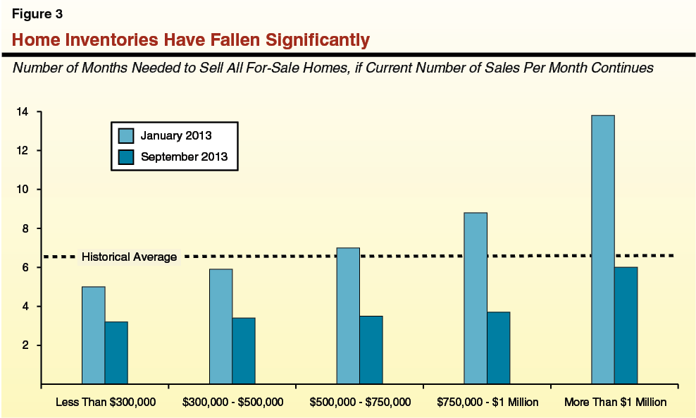
- Cash Investors. Nationwide, 6 million owner–occupied single–family homes converted to rental units over the course of the housing crisis. In most of these cases, investors purchased distressed homes in cash and converted them to rentals, sometimes purchasing hundreds of homes at one time. In Los Angeles, cash purchases as a portion of all home sales increased from 5 percent in 2005 to 34 percent in May 2013, the largest increase in the country. Other areas of California have similarly high all–cash sales rates. Investor demand pushed prices upward—a helpful boost for many distressed areas of the state—but also contributed to reductions in the inventory of owner–occupied homes for sale, which, as shown in Figure 3, has contracted significantly since January 2012.
- Strategic Sellers. The supply of homes for sale depends primarily on the eagerness of current homeowners to sell. Short supplies indicate a general unwillingness or an inability to sell. Unwilling owners may wait to list their homes so as to benefit from expected upward price trends, especially as price gains are accelerating. A national survey of homeowners from earlier this year found that only 25 percent of owners felt it was a good time to sell (whereas two–thirds agreed it was a good time to buy), a sign that potential sellers are waiting. On the other end, more than 15 percent of California homeowners remain underwater on their homes. This means some would–be sellers are unable to do so, keeping a sizable share of the state’s housing stock off the market.
- Cautious Homebuilders. Responding to rising home prices, construction activity has begun to improve. Authorized single–family permits, the first step in constructing a new home, increased from less than 15,000 in the first seven months of 2012 to more than 21,000 in the first seven months of 2013. Though large in percentage terms, this gain represents a historically small response relative to the price increases seen over the same period. (For comparison, the first seven months of 2002 saw 72,000 single–family permits.) In our view, it appears that single–family homebuilders, and, perhaps, their lenders, have remained cautious, wary that increased supply in the short term could dampen prices, threatening the profitability of newly constructed homes. Restricted credit, as well as land–use and development constraints in some areas, also may be holding back some new construction. Until homebuilding quickens, home demand will not be tempered much by new home construction.
Latest Data Suggest Home Prices Are Decelerating to More Normal Trends. Recent price gains appear to be decelerating. Rising mortgage rates and expanding inventories have likely contributed to this deceleration. Interest rates on a 30–year fixed rate mortgage have climbed 1 percentage point since May, equating to a 15 percent increase in the monthly payment on a $200,000 loan. In turn, increased mortgage costs have cooled housing demand. In August and September, home inventories expanded for the first time in a year. These data inform our home price forecast for 2014, which is described below.
We view the pace of recent price gains as unsustainable, and accordingly expect housing inventories to expand as more homeowners feel it is a good time to sell, as cash investor purchases decline, and new housing construction begins to ratchet up, each of which should absorb existing demand and therefore slow price increases. In particular, we expect home price growth to decelerate significantly, to 7 percent in 2014. We project that construction activity, responding to recent price and rent increases, will post strong gains in 2014 (as shown in Figure 4). In 2014, we forecast residential housing permits to increase by 31,000 units to 120,000 permits total. Permits are projected to increase to 136,000 units in 2015 before stabilizing around 160,000 units annually by the end of our forecast period. Compared to past years, multi–family unit permits are projected to make up a larger portion of newly constructed housing stock. Our residential permits forecast has been lowered notably since our prior forecast, released in May 2013, due primarily to our lower expectation for new single–family home construction. We caution, given the sizable shifts taking place in today’s housing market, that actual price gains and construction activity in the coming years could vary widely—either above or below—our office’s forecast over the next few years.
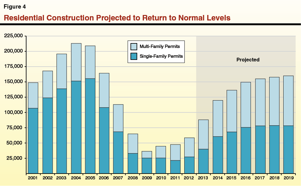
Figure 5 summarizes our November 2013 multiyear General Fund revenue forecast.
Figure 5
LAO November 2013 Revenue Forecast
General Fund and Education Protection Account Combined (In Billions)
|
|
2012–13
|
2013–14
|
2014–15
|
2015–16
|
2016–17
|
2017–18
|
2018–19
|
2019–20
|
|
Personal income tax
|
$65.0
|
$66.0
|
$71.4
|
$75.9
|
$79.6
|
$83.2
|
$82.9
|
$84.1
|
|
Sales and use tax
|
20.5
|
22.8
|
23.6
|
24.9
|
25.4
|
25.8
|
27.0
|
28.2
|
|
Corporation tax
|
7.7
|
8.3
|
8.9
|
9.5
|
10.1
|
10.6
|
11.2
|
11.8
|
|
Subtotals, “Big Three” taxes
|
($93.2)
|
($97.1)
|
($103.8)
|
($110.3)
|
($115.1)
|
($119.6)
|
($121.1)
|
($124.1)
|
|
Insurance tax
|
$2.2
|
$2.2
|
$2.3
|
$2.4
|
$2.5
|
$2.6
|
$2.7
|
$2.8
|
|
Other revenues
|
2.7
|
2.3
|
1.9
|
1.9
|
1.8
|
1.8
|
1.8
|
1.8
|
|
Net transfers and loans
|
1.7
|
0.3
|
–0.4
|
–0.8
|
–0.4
|
0.2
|
0.3
|
0.3
|
|
Totals, Revenues and Transfers
|
$99.8
|
$101.8
|
$107.6
|
$113.8
|
$119.0
|
$124.2
|
$125.8
|
$128.9
|
In June 2013, the Legislature approved the 2013–14 Budget Act. The State Constitution requires the Legislature to determine the revenue estimates underlying each annual budget, so that the budget meets the requirements for a balanced budget in Proposition 58 (2004). In developing the 2013–14 budget, the Legislature considered both our office’s May 2013 revenue forecast, as well as the May 2013 revenue forecast of the administration. Compared to the administration’s forecast, our office’s May 2013 forecast projected $3.2 billion more in General Fund revenues and transfers across the three fiscal years (2011–12, 2012–13, and 2013–14), due principally to our higher assumptions for capital gains–related personal income taxes in 2013 and 2014. The Legislature and the Governor agreed to base the 2013–14 budget plan on the administration’s May 2013 revenue forecast. Figure 6 compares our November 2013 revenue forecasts by fiscal year with those assumed in the 2013–14 budget.
Figure 6
Comparing LAO November 2013 Revenue Forecast With 2013–14 Budget Act Forecast
(General Fund and Education Protection Account Combined, in Millions)
|
|
2012–13
|
|
2013–14
|
|
2013–14 Budget Act Forecast
|
LAO Nov. 2013 Forecast
|
Difference
|
|
2013–14 Budget Act Forecast
|
LAO Nov. 2013 Forecast
|
Difference
|
|
Personal income tax
|
$63,901
|
$65,030
|
$1,129
|
|
$60,827
|
$66,002
|
$5,175
|
|
Sales and use tax
|
20,240
|
20,482
|
242
|
|
22,983
|
22,809
|
–174
|
|
Corporation tax
|
7,509
|
7,669
|
160
|
|
8,508
|
8,278
|
–230
|
|
Subtotals, “Big Three” taxes
|
($91,650)
|
($93,181)
|
($1,531)
|
|
($92,318)
|
($97,089)
|
($4,771)
|
|
Insurance tax
|
$2,156
|
$2,249
|
$93
|
|
$2,200
|
$2,163
|
–$37
|
|
Other revenues
|
2,641
|
2,664
|
23
|
|
2,249
|
2,254
|
6
|
|
Net transfers and loans
|
1,748
|
1,748
|
—
|
|
331
|
342
|
10
|
|
Totals, Revenues and Transfers
|
$98,195
|
$99,841
|
$1,646
|
|
$97,098
|
$101,847
|
$4,749
|
Higher Revenues Now Projected, Compared to 2013–14 Budget Assumptions. Our office’s projections for General Fund revenues in 2011–12, 2012–13, and 2013–14 combined have increased since May by over $3 billion. As shown in Figure 6, we now project that General Fund revenues and transfers for 2011–12, 2012–13, and 2013–14 combined will be $6.4 billion higher than the amounts assumed in the 2013–14 state budget plan. For 2012–13, state collections exceeded forecasts. For 2013–14, most of the increase in our forecast since May results from higher assumptions concerning capital gains and some other categories of taxable income attributable largely to higher–income personal income tax (PIT) filers. Our increased capital gains assumptions result primarily from stronger stock market and real estate market performance since May.
PIT Collections Running Stronger Than 2013–14 Budget Act Forecast. In 2012–13, revenue collections were stronger than projected by either our office or the administration in May 2013. Through the end of October, 2013–14 PIT estimated payments—tied in large part to capital gains and business income—have exceeded the administration’s monthly projections by 34 percent. Several key PIT payment dates remain during the fiscal year, but to date, the available information suggests that PIT revenues are running considerably stronger than was assumed in the budget act.
Uncertainty remains, however, given that 2012 income tax collections were elevated for a variety of reasons, as discussed below, and preliminary tax agency data on what was reported on 2012 PIT returns will not begin to be made available until a few weeks from now. (Final tax agency data related to 2012 returns will not be available until several months from now.) Moreover, the performance of the stock market has been much stronger than our office assumed in May, and stock performance in the coming few weeks will affect 2013 capital gains to some extent. Uncertainty also results from the state’s complicated revenue accrual methodologies, which move some PIT and other revenues from one fiscal year to a prior one for budgetary accounting purposes.
Legislative Action Needed to Oversee Complex Accrual Process
Prior–Year Revenue Estimates Now Change for at Least Two Years Thereafter. As the 2014–15 budget process begins, we think it is important to emphasize that, under the new “net final payment” accrual process authorized in recent annual budgets for Proposition 30 revenues, personal income tax revenues essentially are still changing for 2011–12. As we understand the accrual process, 2011–12 revenue estimates should keep changing until at least May 2014, given that estimates of 2012 capital gains—a key driver of Proposition 30 revenues for that year—will change until at least that point in time, as tax agencies review and “sample” for statistical purposes more and more 2012 tax returns. Total 2012–13 revenues will change until May 2015, and so on. Even as legislators make budget decisions and weigh various uncertainties about 2013–14 and 2014–15 revenue and spending, they may know less than ever before about the previous two fiscal years’ budget results and the state budget reserves remaining therefrom. We acknowledge that our revenue estimates may be too high or too low by hundreds of millions of dollars per year—or, in some scenarios, over $1 billion per year—due simply to the challenges we face in making projections concerning this complex part of the budget process.
Revenue Calculations Will Affect Future Budgeting. If the administration follows its past practice, it will not display in its 2014 budget publications up–to–date estimates of 2011–12 revenues based on these accrual changes. Based on past practice, 2011–12 revenues would have been “closed” in 2013. Any changes to prior–year revenues—often minor under past accrual policies—would be listed, along with many expenditure reconciliations, as changes to the incoming General Fund balance. If the administration sticks to this past practice, the Legislature will lack complete, transparent access to information that would be important to budgeting—especially information that will help them decide whether Proposition 98 obligations have been appropriately estimated.
We recommend that the Legislature require the administration to display publicly for budgetary decision–making purposes the adjusted prior–year revenue amounts included in its adjustments to the incoming General Fund balance. Such prior–year revenue changes should be incorporated in all historical documents related to state revenues—otherwise, the reliability of that historical data could decline significantly. Finally, we recommend that the Legislature require the administration—at least once a year on its website—to describe in plain English each of the calculations used to move revenue from one fiscal year to a prior year via the accrual process.
2012–13 PIT Collections Were Elevated . . . PIT collections grew substantially in 2012–13 due to voters’ approval of Proposition 30, large one–time withholding payments related to the initial public offering (IPO) of stock by Facebook, Inc., and one–time accelerations of various types of income in 2012 by high–income taxpayers—especially accelerated realizations of capital gains. (Such accelerations of income allowed some taxpayers to avoid higher federal tax rates that went into effect for some in 2013.) For tax year 2012, by our office’s estimation, capital gains seem to have produced slightly over $10 billion of revenue for the state—around 15 percent of the current annual PIT base. We now estimate that 2012–13 PIT revenues will end higher than the levels projected in both the LAO and administration May 2013 forecasts. Specifically, our current estimate of 2012–13 PIT revenues—$65 billion—is $1.1 billion above the 2013–14 Budget Act assumption, which was based on the administration’s May 2013 forecast.
. . . Which Means PIT Growth to Be Much Slower in 2013–14 . . . In our May 2013 Forecast, we projected that PIT collections would fall by 0.2 percent in 2013–14—an unusual assumption since PIT revenues typically fall only in recession years. Because so much income was accelerated from 2013 to 2012 to avoid higher federal taxes, we assumed that net capital gains realizations by California residents would fall by 30 percent in 2013, affecting both estimated payments in late 2013 and January 2014. Since May, however, the performance of the stock market has exceeded our prior assumptions. While we continue to assume a large drop in net capital gains realized by California taxpayers in 2013, our capital gains assumption for that year is now a few percentage points higher than it was in May. Moreover, our 2014 capital gains assumption—which also affects 2013–14 PIT collections—has risen by over 10 percent, given the recent growth in stock prices. Our new forecast also assumes stronger growth for PIT withholding—revenue collections that result mainly from Californians’ wage income. This assumption seems more consistent with recently strong year–over–year PIT withholding growth (after adjusting for the one–time withholding payments resulting from the Facebook IPO in October 2012). After accounting for accruals, we now forecast that 2013–14 PIT revenues will rise by 1.5 percent to $66 billion. This is $5.2 billion above the amount assumed in the budget approved in June.
. . . And PIT Should Bounce Back in 2014–15. The acceleration of large amounts of revenue from 2013 to 2012 artificially depresses growth in PIT revenues in 2013–14. Accordingly, both our office’s forecast and the administration’s forecast have projected that the growth rate for PIT revenues will bounce upward in 2014–15. In this forecast, we project that PIT revenues grow by 8 percent to $71 billion in 2014–15.
2015–16 and Beyond. Our forecast assumes roughly 5 percent average annual growth in PIT revenues between 2015–16 and 2017–18. This rate of annual growth is consistent with what we would expect in a mature economic expansion—such as that assumed in our multiyear economic forecast through 2020—accompanied by some growth in stock and house prices. We then project much slower growth in 2018–19 and 2019–20 due primarily to the expiration of Proposition 30’s higher PIT rates for high–income taxpayers at the end of 2018. This means that the PIT revenue loss from Proposition 30’s expiration will not occur all at once, but instead will be spread over those two fiscal years. We now project that PIT revenues will fall by 0.4 percent in 2018–19 to under $83 billion before rising by 1.4 percent in 2019–20 to $84 billion.
PIT Revenues Make Up Bigger Percentage of General Fund Than Ever Before. Prior to the first fiscal year affected by Proposition 30, the PIT’s share of total General Fund revenues and transfers had exceeded 60 percent only once—at the end of the “dot–com” bubble in 2000–01. We are now projecting that PIT revenues will comprise two–thirds of total General Fund revenues in 2014–15—the highest such percentage recorded to date in California history. Proposition 30—with its temporary marginal tax rate increases for high–income households—has increased PIT revenues recently. The percentage of the budget paid for from PIT revenues also has risen recently due to other tax policy changes. Specifically, the shift of a portion of the state’s sales and use tax (SUT) from the General Fund to local realignment accounts and a few other changes have reduced the percentage of the General Fund paid from other revenue sources, thereby increasing the share of the General Fund paid by the PIT. Finally, the amount of taxable income received by the top 20 percent of taxpayers has, in real terms, grown much faster than the amounts for middle–income and lower–income taxpayers in recent decades. As these higher–income taxpayers pay the highest marginal tax rates, the increasing concentration of income in that group tends to generate significant growth in PIT revenues over time.
Our forecast projects that PIT will maintain that two–thirds share of annual General Fund revenues. (As our forecast assumes a fairly modest level of capital gains—compared to the size of the economy—in future years, this amount could be higher in particularly strong capital gains years, and it could be weaker when capital gains are very low.) We note, however, that the proportion of the General Fund supported by PIT revenues likely would be growing even if Proposition 30 were not in effect due to more income concentration among the highest–income taxpayers and the other factors described earlier.
Higher Stock Market Driving Higher PIT Projections in the Near Term. The change from year to year in the state’s net capital gains has proven over time to be closely correlated with changes in stock and house prices, as well as stock trading volume. Recently, both stock and house prices have been growing rapidly. Our office’s May 2013 forecast assumed that the S&P 500 index remained close to its May 14, 2013 level of 1650 through the rest of 2013. As of October 25, when we finalized our economic assumptions for this forecast, it closed at 1760 (7 percent above our prior assumptions). This is the key reason for the higher capital gains in our forecast in the near term and a major reason for our higher forecast of 2013–14 PIT revenues.
Stock Market Valuations Near Historical Norms. In general, key stock market valuation metrics—such as the price–to–earnings (PE) ratio for the S&P 500—are in line with historical norms. Some such metrics are somewhat above norms, and some are below. We note, however, that PE ratios are considerably below the levels experienced during the dot–com bubble, when Californians’ net capital gains realizations peaked as a percentage of personal income in the state at 10.6 percent. Our forecast assumes that net capital gains total 5.9 percent of personal income in 2012, 4.3 percent in 2013 (lower due to the income accelerations described earlier), and 6 percent in 2014. This incorporates an assumption that stock prices remain stable—at or near their October 25 level—through March 2014. Thereafter, we assume that stock prices grow slower than the overall growth of the U.S. economy, which results in net capital gains falling to 4.4 percent of personal income by the end of our forecast period in 2020. This forecasting assumption is intended, in the context of the economic expansion we assume through 2020, to keep stock prices near historical norms throughout the period.
Volatile Stock Prices Certainly Cannot Be Predicted With Precision. Because PIT is the state’s largest revenue source, and a significant, volatile portion of that tax is generated from capital gains on the sales of stocks and other assets, every forecast of California’s public finances must reflect an assumption—either explicit or implicit—about the direction of the stock market. Our forecasting methodology attempts to use the most realistic assumptions possible about stock performance in the near term and, to the extent that these assets seem overpriced relative to historical norms, to bring them closer to those norms over time. Currently, there is not clear evidence that stocks are overpriced significantly compared to those norms. Accordingly, we assume stable stock prices in the near term and modest growth thereafter.
Nevertheless, over any given forecast period—even the next few quarters—stock prices can be expected to differ from any set of assumptions. They may be lower in some periods, and they may be higher in others. This volatility—as well as fundamental changes in stock prices that occur during bull and bear markets—may cause actual capital gains to differ significantly from any forecast. In the near term, for example, annual PIT revenues can be $2 billion higher or lower than forecast based on differing capital gains results alone. (Other forecasting differences could produce additional changes in revenues.) State leaders should consider all of this information when making budgetary commitments and determining the level of financial reserves for the state to have at any given time.
Estimated General Fund SUT revenue totaled $20.5 billion in 2012–13, about $240 million higher than the amount assumed in the 2013–14 budget. In 2013–14, we expect SUT receipts to increase by 11 percent to $22.8 billion (about $170 million below the 2013–14 budget assumption). The projected growth in 2013–14 reflects (1) the full–year effect of Proposition 30’s temporary one–quarter cent SUT increase and (2) projected growth in underlying taxable sales of 6.9 percent. In 2014–15, we forecast SUT revenue to increase by 3.3 percent to $23.6 billion. This lower revenue growth is largely due to the new tax credit for manufacturing equipment established by Chapter 69, Statutes of 2013 (AB 93, Committee on Budget), which begins in 2014–15. (Underlying revenue growth—that is, without the impacts of the credit—is 5.4 percent, in line with projected growth in taxable sales.) Projected SUT revenues then increase by 5.6 percent in 2015–16 before growing more slowly over the following two years as the one–quarter cent Proposition 30 SUT increase expires at the end of 2016. Revenue growth stabilizes towards the end of our forecast, closely tracking projected growth in taxable sales.
Housing Permits Play a Major Role in the Sales Tax Forecast. The main determinant of SUT receipts is taxable sales. For a variety of reasons, taxable sales and housing permits tend to move together, making housing permits a useful economic indicator for forecasting taxable sales. House construction generates some taxable sales directly (through purchases of construction materials and other goods), but it also acts as a proxy for consumer confidence, which is difficult to measure directly. As a result, housing permits can account for year–to–year variation in taxable sales that cannot be explained by variation in personal income or nationwide retail sales. For taxable sales and housing permits, we project significant growth from 2012–13 to 2013–14 and slower growth thereafter. Specifically, we expect taxable sales to grow about 7 percent in 2013–14 before falling to below 5 percent later in the forecast period. Similarly, we expect housing permits to grow by 36 percent from 2013 to 2014, with slower growth in later years.
2011 Realignment and Other Local Sales Taxes. Roughly half of California’s sales tax revenue is distributed to counties, cities, and special districts through various mechanisms, including the funding stream established to support the 2011 realignment plan. Some factors that affect the growth in state General Fund sales tax revenue—such as the Proposition 30 quarter–cent SUT rate increase and the new sales tax exemption for certain equipment purchases—do not affect local sales tax revenues. Instead, growth in taxable sales is the primary driver of changes in local sales tax revenue. As shown in Figure 7, we expect steady growth in 2011 Local Revenue Fund sales tax revenue despite the fluctuations in General Fund sales tax revenue. Specifically, we estimate that 2011 realignment sales tax revenues will grow by 7 percent in 2013–14 and by 5.4 percent in 2014–15. Annual growth in these revenues is expected to increase slightly to 5.5 percent in 2015–16 and then decelerate to 4.4 percent by the end of the forecast period.
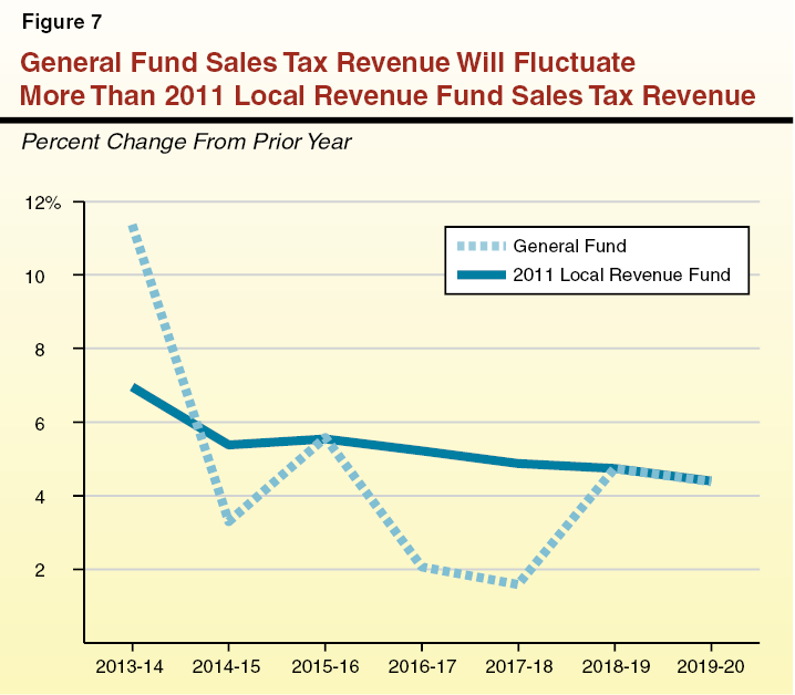
Estimated General Fund corporation tax (CT) revenue totaled $7.7 billion in 2012–13, $160 million above the 2013–14 Budget Act assumption. We forecast that CT revenue will increase to $8.3 billion in 2013–14, $230 million below the budget act assumption. Thereafter, our forecast projects that CT revenue will increase steadily, reaching $11.8 billion in 2019–20. This reflects an average annual growth rate of 6 percent.
Forecasting Complicated by Continued Uncertainty. As we have noted in prior years, the Legislature and voters (with passage of Proposition 39) have recently enacted major changes in business tax policy that have drastically changed the relationships between economic and tax data. In the near term, it is easy to imagine actual annual revenues for this tax being hundreds of millions of dollars higher or lower than our forecast in any given year. It may take several years before data is available to help us address these forecasting uncertainties.
Nationally, Corporate Profits Have Recovered . . . The vast majority of California CT revenue is paid by large multistate and multinational corporations that apportion (allocate) a share of their profits to California. Corporate profits, both nationally and in California, declined significantly during the 2007–2009 recession. National corporate profits, as estimated by the Bureau of Economic Analysis, have recovered to their prerecession levels and then some. Further, our forecast assumes that U.S. profits will grow by 12 percent in 2014.
. . . But California CT Revenues Remain Depressed. Taxable corporate profits apportioned to California have recovered somewhat but have not returned to their prerecession levels. Despite the strong growth trend in U.S. profits, California CT revenues have declined in several recent years. The precise reasons for this are likely varied and will take more time to assess. The weakness in California CT collections is partially the result of budget actions passed by the Legislature in recent years to collect revenues earlier and delay the use of certain tax credits and deductions. These measures had the net effect of moving revenue forward to 2008–09 and 2009–10 from future years. While the effects of some of these measures may have run their course, the state is only now beginning to feel the full impact of others, such as the suspension of net operating loss (NOL) deductions. In addition, in 2011 and 2012 corporations were permitted to choose their preferred method for allocating profits to California. We tentatively estimate that this reduced the CT base by about 13 percent in 2011 and 2012. Proposition 39 changed this policy by requiring most corporations to use the “single sales factor” method of apportioning multistate and multinational profits to taxation in California beginning in 2013. (The Franchise Tax Board is unlikely to be able to determine the impact of Proposition 39 with precision until the spring of 2015, when preliminary CT data for tax year 2013 becomes available.) If the net revenue change resulting from all of these apportionment changes is negative, this could help explain some of the recent weakness in CT collections.
NOL Deductions Assumed to Increase Tenfold in 2012. The use of NOL deductions—in which corporations deduct a prior loss from current tax year profits—were suspended for most corporations for tax years 2008–2011. As a result, 2012 was the first year in which large corporations were able to use NOL deductions since the recession. We assume that increasing profits will be somewhat offset by widespread use of NOL deductions. Our forecast assumes that $30 billion in NOLs were deducted in tax year 2012, declining to around $21 billion per year by 2020. Should this level of NOL deductions not materialize, CT revenue could exceed our forecast. On the other hand, a higher level of NOL deductions could reduce CT revenue.
Use of Tax Credits Projected to Increase. As profits continue to increase, businesses will be more able to use new or previously generated tax credits to reduce taxes owed. We assume that businesses will use a total of $3 billion in tax credits in 2013 and that this level steadily rises to a total of $3.5 billion in 2020. Increases of CT credit usage are slowed, compared to what they would be otherwise, by our assumptions related to the replacement of enterprise zones with different tax provisions. The research and development tax credit accounts for the majority of the credits used to offset CT liability. We assume that businesses will use about $2.3 billion in research and development tax credits in 2013 and that this will rise to $3.2 billion by 2020.
LAO Forecast Assumes Current–Law Special Fund Repayments. In recent years, to help balance the General Fund budget, the Legislature approved billions of dollars of loans from several dozen of the state’s special funds—funds for specific programs that are often supported by dedicated fee revenues related to the programs themselves. As of the end of 2012–13, $4.6 billion of these loans remained outstanding. Payments to retire the principal amounts of these loans are booked as transfers out of the General Fund, so that when the state repays significant amounts of such loans, the net transfers and loans displayed in Figure 5 tend to be a negative amount. Some special fund loans have specific repayment dates in prior budget acts, and, consistent with case law, it is state practice to repay funds in cases when they have an imminent fiscal need for such repayment. Based on these criteria, our forecast assumes $696 million of special fund loan repayments in 2013–14, $630 million in 2014–15, $1 billion in 2015–16, $660 million in 2016–17, and $100 million in 2017–18. Thus, in our forecast showing future state surpluses, we assume—consistent with these criteria—that $1.5 billion of special fund loans remain outstanding as of the end of the 2019–20 fiscal year.
The Governor’s wall of debt proposal anticipates a faster retirement of special fund loans than indicated in our forecast. His proposal would make special fund loan repayments the focus of the Legislature’s discretionary, non–Proposition 98 wall of debt payments over the next few years. Specifically, the Governor would dedicate about $1 billion more of General Fund resources to special fund repayments through 2016–17—principally in 2015–16. If the Legislature were to adopt the Governor’s proposal, therefore, this would reduce the operating surpluses displayed in some years of our forecast, especially in 2015–16. (The approach we discuss in Chapter 1 for using possible General Fund surpluses would repay all special fund loans—and other parts of the wall of debt—within a few years.)
In this chapter, we discuss our estimates of spending for 2012–13 and 2013–14, as well as our spending projections for 2014–15 through 2019–20. Figure 1 displays our expenditure forecast for the General Fund and the Education Protection Account (EPA) created by Proposition 30 (2012).
Figure 1
Projected General Fund and Education Protection Account Spending
(Dollars in Millions)
|
|
Estimates
|
|
Forecast
|
Average Annual Growtha
|
|
2012–13
|
2013–14
|
|
2014–15
|
2015–16
|
2016–17
|
2017–18
|
2018–19
|
2019–20
|
|
Education programs
|
|
Proposition 98
|
$42,212
|
$42,123
|
|
$45,409
|
$47,414
|
$47,448
|
$48,747
|
$48,627
|
$49,103
|
2.6%
|
|
QEIA payment
|
—
|
—
|
|
410
|
—
|
—
|
—
|
—
|
—
|
—
|
|
Child Care
|
751
|
742
|
|
756
|
778
|
804
|
844
|
885
|
925
|
3.7
|
|
CSU
|
1,991
|
2,242
|
|
2,242
|
2,242
|
2,242
|
2,242
|
2,242
|
2,242
|
0.0
|
|
UCb
|
2,166
|
2,844
|
|
2,844
|
2,844
|
2,844
|
2,844
|
2,844
|
2,844
|
0.0
|
|
CSAC
|
708
|
1,039
|
|
1,162
|
1,206
|
1,370
|
1,448
|
1,453
|
1,459
|
5.8
|
|
Health and Social Services
|
|
Medi–Cal
|
14,929
|
16,255
|
|
16,509
|
17,127
|
18,757
|
20,050
|
21,336
|
23,048
|
6.0
|
|
CalWORKsc
|
1,521
|
1,195
|
|
716
|
651
|
602
|
565
|
536
|
509
|
–13.2
|
|
SSI/SSP
|
2,753
|
2,787
|
|
2,825
|
2,865
|
2,906
|
2,948
|
2,991
|
3,036
|
1.4
|
|
IHSS
|
1,772
|
1,842
|
|
1,893
|
1,996
|
2,070
|
2,139
|
2,209
|
2,280
|
3.6
|
|
DDS
|
2,648
|
2,789
|
|
2,951
|
3,088
|
3,230
|
3,336
|
3,446
|
3,560
|
4.2
|
|
DSH
|
1,278
|
1,408
|
|
1,445
|
1,451
|
1,458
|
1,465
|
1,471
|
1,471
|
0.7
|
|
Otherd
|
1,458
|
1,465
|
|
1,520
|
1,554
|
1,578
|
1,590
|
1,602
|
1,615
|
1.6
|
|
CDCR
|
8,347
|
8,746
|
|
8,702
|
8,808
|
8,819
|
8,864
|
8,912
|
8,960
|
0.4
|
|
Judiciary
|
750
|
1,184
|
|
1,199
|
1,191
|
1,182
|
1,174
|
1,165
|
1,154
|
–0.4
|
|
Infrastructuree
|
4,677
|
5,156
|
|
5,790
|
6,299
|
6,399
|
6,952
|
6,899
|
7,056
|
5.4
|
|
Other programs
|
9,391
|
7,823
|
|
8,062
|
8,709
|
8,989
|
9,327
|
9,584
|
9,821
|
3.9
|
|
Totals
|
$97,352
|
$99,639
|
|
$104,436
|
$108,224
|
$110,698
|
$114,535
|
$116,205
|
$119,085
|
3.0%
|
|
Percent change
|
—
|
2.3%
|
|
4.8%
|
3.6%
|
2.3%
|
3.5%
|
1.5%
|
2.5%
|
—
|
Higher Revenue Forecast Increases Proposition 98 Spending. As discussed in Chapter 2, our forecast of General Fund revenues for 2011–12, 2012–13, and 2013–14 combined is about $6.4 billion higher than the 2013–14 budget assumptions. As described below, this results in about $4.8 billion in higher General Fund Proposition 98 spending in 2012–13 and 2013–14 combined. In total, our spending estimates for 2012–13 and 2013–14 combined are $5 billion higher than the 2013–14 budget assumptions, 2.6 percent above the combined enacted total for those years.
Spending Projected to Slow Considerably Near End of Forecast. We project spending to grow at an average annual rate of 3 percent from 2013–14 through 2019–20. Spending is projected to slow considerably in the outer years of the forecast. This is principally due to healthy growth in local property taxes and the end of the “triple flip,” both of which reduce General Fund spending necessary to meet the Proposition 98 minimum guarantee. Across the rest of the budget, we project that Medi–Cal spending will grow at an average annual rate of 6 percent from 2013–14 through 2019–20. Growth in Cal Grants spending (5.8 percent annually) is almost entirely due to implementation of a new scholarship program beginning in 2014–15. As discussed later in this chapter, spending on California Work Opportunity and Responsibility to Kids (CalWORKs) is projected to decline at a yearly rate of 13.2 percent during the forecast period due largely to a decision in the 2013–14 budget to offset a significant portion of General Fund program costs with certain realignment funds. General Fund spending on Proposition 98—the single largest state program—is projected to grow at only 2.6 percent a year over the period. Total Proposition 98 spending, however, grows at the more rapid annual pace of 4.1 percent, as property tax revenues are assumed to grow at healthy rates over the period.
Overview of Education Forecasts. Below, we discuss three education–related expenditure projections. Our Proposition 98 forecast projects spending for preschool, elementary, and secondary education (commonly referred to as K–12 education), and the California Community Colleges. Our higher education forecast projects spending for the California State University (CSU), the University of California (UC), Hastings College of the Law, and state financial aid programs. Our child care forecast projects spending on subsidized care for CalWORKs families and other low–income working families.
Proposition 98 “Minimum Guarantee” for Schools and Community Colleges. State budgeting for schools and community colleges is governed largely by Proposition 98, passed by voters in 1988. The measure, modified by Proposition 111 in 1990, establishes a minimum funding requirement, commonly referred to as the minimum guarantee. Both state General Fund (including EPA) and local property tax revenue apply toward meeting the minimum guarantee. In addition to Proposition 98 funding, schools and community colleges receive funding from the federal government, other state sources (such as the lottery), and various local sources (such as parcel taxes).
Calculating the Minimum Funding Guarantee. The Proposition 98 minimum guarantee is determined by one of three tests set forth in the State Constitution. These tests are based on several inputs, including changes in K–12 average daily attendance, per capita personal income, and per capita General Fund revenue. Though the calculation of the minimum guarantee is formula–driven, a supermajority of the Legislature can vote to suspend the formulas and provide less funding than the formulas require. This happened in 2004–05 and 2010–11. In some cases, including suspensions, the state creates a future obligation referred to as a “maintenance factor.” The state is required to make maintenance factor payments when year–to–year growth in state General Fund revenues is relatively strong, such that increases in education funding are accelerated. The state can always provide more than the minimum guarantee in any given year.
Minimum Guarantee $1.7 Billion Higher in 2012–13. Figure 2 compares our updated estimates of the minimum guarantee in 2012–13 with what was assumed for that year at the time the 2013–14 spending plan was enacted. As the figure shows, we estimate the minimum guarantee has increased $1.7 billion. The increase results from our estimate that 2012–13 General Fund revenues are $1.6 billion higher than assumed in the spending plan. The higher state revenues result in more than a dollar–for–dollar increase in the Proposition 98 minimum guarantee because of the way the state has decided to make maintenance factor payments when Test 1 is operative. In total the state will be making a $5.4 billion maintenance factor payment in 2012–13 (leaving $5.6 billion in outstanding maintenance factor).
Figure 2
Increases in 2012–13 and 2013–14 Minimum Guarantees
(In Millions)
|
|
2012–13
|
|
2013–14
|
|
2013–14 Budget Plan
|
November LAO Forecast
|
Change
|
2013–14 Budget Plan
|
November LAO Forecast
|
Change
|
|
Minimum Guarantee
|
|
|
|
|
|
|
|
|
General Fund
|
$40,454
|
$42,212
|
$1,758
|
|
$39,055
|
$42,123
|
$3,068
|
|
Local property tax
|
16,011
|
15,994
|
–17
|
|
16,226
|
15,833
|
–393
|
|
Totals
|
$56,465
|
$58,206
|
$1,741
|
$55,281
|
$57,956
|
$2,675
|
Minimum Guarantee $2.7 Billion Higher in 2013–14. Also shown in Figure 2, we project the 2013–14 minimum guarantee to be $58 billion—$2.7 billion higher than the 2013–14 Budget Act estimate. The higher minimum guarantee is primarily due to our projected increase in the year–to–year growth of General Fund revenues. Although the minimum guarantee increases by $2.7 billion, General Fund Proposition 98 spending increases by $3.1 billion as a result of our local property tax forecast being $393 million lower than the budget act estimate. We forecast redevelopment agency (RDA) property tax revenues will be $332 million lower, while other local property tax revenues will be $61 million below budget act estimates. In 2013–14, we estimate that $941 million in maintenance factor will be created (bringing the state’s outstanding maintenance factor up to $6.8 billion). The 2013–14 budget plan assumed $2.6 billion in maintenance factor was created, but the amount has decreased due to the stronger projected growth in General Fund revenues.
Additional 2012–13 and 2013–14 Funding Can Be Used to Pay Down Outstanding Obligations. We estimate that the minimum guarantees for 2012–13 and 2013–14 will be up a combined $4.4 billion. Given the 2012–13 school year has been completed and the 2013–14 school year is underway, the additional funding in practical terms is available for one–time purposes, including paying down the state’s still sizeable outstanding school and community college obligations. Of the $11.5 billion in outstanding Proposition 98 obligations, the state has $6.2 billion in outstanding deferrals, $4.8 billion in unpaid mandate claims, and $462 million owed for the Emergency Repair Program (ERP). Using the additional 2012–13 and 2013–14 funds for these purposes would reduce the state’s outstanding obligations by almost 40 percent.
Paying Down Different Types of Obligations Has Different Distributional Effects. Paying down deferrals would provide some benefit to most districts (about 850 of 958 school districts and 68 of 72 community college districts), but districts that rely most heavily on state funding would receive the greatest benefit. These districts tend to be ones that have low property values or are located in counties that historically have distributed a greater share of property tax revenues to cities, counties, and special districts. By having state payments provided to them on schedule, these districts’ cash flow situations would improve and they would have less need to borrow either internally or externally.
Paying down the mandate backlog also would benefit virtually all school and community college districts but would have different distributional effects. This is because some districts file more claims and claim much higher costs (in per–pupil terms) than other districts. In addition, school districts serving high school students would benefit greatly from the state’s pay–off of the high school graduation requirements mandate. All school districts would be eligible to benefit notably from the pay–off of the Behavioral Intervention Plan mandate. In all these cases, as school and community college districts already paid the costs associated with the original mandated activities, they benefit from additional general purpose funds that they could use for any high–priority, one–time purpose. For example, school districts could use the funding to help further implement the Common Core State Standards or address deferred maintenance.
Paying down the ERP obligation would affect only those schools in the bottom three deciles of the state’s academic accountability index that filed repair requests with the Office of Public School Construction several years ago. (Schools no longer can submit applications, as previously approved projects exceed the amount owed for the program.) Given these schools likely already undertook the emergency repairs, they would be able to use new ERP funding for any current high–priority, one–time purpose (including other maintenance needs).
2014–15 Guarantee $4.2 Billion Higher Than Updated 2013–14 Guarantee. Our forecast projects a minimum guarantee of $62.2 billion in 2014–15. This is a $4.2 billion increase from our projected 2013–14 minimum guarantee. The increase in the guarantee is driven primarily by the year–to–year growth in General Fund revenues. We project that Test 1 will be operative in 2014–15 and a large maintenance factor payment will be required ($3.6 billion). This large maintenance factor payment is a result of a projected decline in per capita personal income (–0.8 percent) coupled with a large projected increase in per capita General Fund revenues (6.4 percent). (The maintenance factor payment is driven primarily by the difference between these two factors, with the payment increasing as growth in General Fund revenues outpaces growth in personal income.) This situation is very similar to what the state faced in 2012–13, with the minimum guarantee and the required maintenance factor payment very sensitive to changes in General Fund revenues.
2014–15 Guarantee Almost $8 Billion Higher Than Current Ongoing Programmatic Spending Level. As Figure 3 shows, of the $55.3 billion in Proposition 98 funding the state provided in the 2013–14 spending plan, it designated almost $900 million for one–time purposes, leaving $54.4 billion for ongoing purposes. Hence our estimate of the 2014–15 minimum guarantee is almost $8 billion (14 percent) higher than the current ongoing Proposition 98 spending level.
Figure 3
Considerable New Proposition 98 Funding Projected for 2014–15
(In Millions)
|
2013–14 Budget Act Spending Level
|
$55,281
|
|
Back out one–time actions:
|
|
|
Deferral pay downs
|
–272
|
|
Common Core implementation
|
–250
|
|
Career Pathways program
|
–250
|
|
Governor vetoes
|
–35
|
|
CCC building maintenance
|
–30
|
|
CCC adult education planning grants
|
–25
|
|
CCC technology initiative adjustment
|
–7
|
|
Total One–Time Actions
|
–$869
|
|
2013–14 Ongoing Spending
|
$54,412
|
|
New Funds Available in 2014–15
|
$7,748
|
|
2014–15 Minimum Guarantee
|
$62,160
|
Balancing One–Time and Ongoing Spending Key to 2014–15 Budget Planning. Given such a large projected year–to–year funding increase, we recommend the Legislature use the additional funds for a combination of one–time and ongoing purposes. The state, for example, could provide roughly half (about $4 billion) for one–time purposes (including further paying down existing one–time obligations) and roughly half for ongoing purposes. Under this approach, K–12 per–pupil programmatic funding still would increase about $600 (7 percent) year over year. Balancing one–time and ongoing spending in 2014–15 can help districts plan for and accommodate programmatic growth. It also can minimize the adverse effect on schools and community colleges if General Fund revenues do not materialize as expected (due either to an economic slowdown or typical volatility in revenues from capital gains). This is of particular concern in 2014–15 given the guarantee would be extremely susceptible to swings in revenues (as described above). If revenues fall short in 2014–15, one–time funding could be rescinded with minimal or no effect on ongoing school and community college programs. If revenues fall short in 2015–16, ongoing programs also would experience little or no reduction, as the prior–year one–time funding commitments would impose no ongoing cost pressure. That is, the state’s decision to moderate ongoing programmatic commitments in 2014–15 would make having to cut those programs less likely the following year in the event General Fund revenues came in weaker than projected.
Slower Growth When Proposition 30 Revenues Expire. Figure 4 displays our estimates of the minimum guarantee throughout the forecast period. As the figure shows, we project annual increases in the minimum guarantee of about $3 billion from 2015–16 through 2017–18. In 2018–19 and 2019–20, we project more modest annual growth in the minimum guarantee as the PIT revenues enacted by Proposition 30 phase out over 2018–19 and 2019–20.
Figure 4
Proposition 98 Forecast
(Dollars in Billions)
|
|
2014–15
|
2015–16
|
2016–17
|
2017–18
|
2018–19
|
2019–20
|
|
Minimum Guarantee
|
|
|
|
|
|
|
|
General Fund
|
$45.4
|
$47.4
|
$47.4
|
$48.7
|
$48.6
|
$49.1
|
|
Local property tax
|
16.8
|
17.9
|
20.6
|
21.9
|
23.1
|
24.6
|
|
Totals
|
$62.2
|
$65.3
|
$68.1
|
$70.7
|
$71.7
|
$73.7
|
|
Year–to–Year Change in Guarantee
|
|
|
|
|
|
|
|
Amount
|
$4.2
|
$3.2
|
$2.8
|
$2.6
|
$1.1
|
$1.9
|
|
Percent change
|
7.3%
|
5.1%
|
4.2%
|
3.8%
|
1.5%
|
2.7%
|
|
Proposition 98 Obligations
|
|
|
|
|
|
|
|
Maintenance factor created/paid (+/–)
|
–$3.6
|
–$0.2
|
—
|
$0.6
|
$2.1
|
$1.3
|
|
Outstanding maintenance factor
|
3.2
|
3.1
|
$3.2
|
3.9
|
6.2
|
7.8
|
|
Key Factors
|
|
|
|
|
|
|
|
Proposition 98 “Test”
|
1
|
2
|
3
|
3
|
3
|
3
|
|
K–12 average daily attendance
|
–0.1%
|
–0.2%
|
–0.3%
|
–0.4%
|
–0.3%
|
–0.3%
|
|
Per capita personal income (Test 2)
|
–0.8
|
4.9
|
4.6
|
5.0
|
4.8
|
4.8
|
|
Per capita General Fund (Test 3)
|
6.4
|
5.8
|
4.1
|
3.7
|
1.1
|
2.3
|
|
K–14 cost–of–living adjustment
|
0.9
|
2.2
|
2.3
|
2.6
|
2.6
|
2.5
|
School Property Taxes Grow Quickly Over Forecast Period. Over the next several years, we project underlying local property taxes to grow, on average, about 7 percent each year. Though above levels seen in recent years, our estimates are in line with average historical growth. In addition to growth from underlying local property taxes, a couple of specific factors will result in additional school property tax growth in the coming years. First, we project that school and community college property tax revenues will increase by $1.6 billion, beginning in 2016–17, after the state’s Economic Recovery Bonds—approved by voters in 2004 to help close the state budget gap—are repaid. (Under the so–called triple flip, the state effectively diverted local sales taxes to pay off the bonds and reimbursed cities and counties with school and community college property taxes. The state then automatically backfilled the lost property tax revenues to schools and community colleges with additional Proposition 98 General Fund revenues. With the end of the triple flip, these local property tax revenues will return to schools and colleges.) Second, we project that residual RDA property tax revenues—the amounts left over after RDAs pay their various obligations—increase from $763 million in 2013–14 to $1.9 billion in 2019–20. The growth in residual RDA revenues is somewhat offset by the steady decrease in revenues from RDA assets. We forecast schools and community colleges will receive $402 million in RDA asset revenues in 2013–14, with decreases annually through 2017–18 and no RDA asset revenues projected thereafter.
Increases in Guarantee Largely Covered by Local Property Tax Growth. Over the last four years of the forecast period, we project the minimum guarantee increases by $5.6 billion, yet the General Fund contribution to Proposition 98 increases only $1.7 billion. This is because local property tax revenues received by schools and community colleges apply towards meeting the minimum guarantee, such that increases in this revenue stream typically reduce the state’s Proposition 98 General Fund contribution. Given the strong projected growth in property tax revenues described above, the state’s General Fund Proposition 98 requirement bears little of the growth in the guarantee over this period. Absent this growth in property tax revenues, the state’s General Fund costs would be notably higher over the forecast period and would result in significantly lower budgetary surpluses.
State Could Make Progress but Likely Not Fully Implement LCFF by End of Forecast Period. The administration estimated the state could afford to fully implement the Local Control Funding Formula (LCFF) for county offices of education (COEs) by 2014–15 and the LCFF for school districts by 2020–21. Under our forecast, the state would meet its time frame for COEs but likely would be unable to meet the time frame for school districts, even given the projected increases in the minimum guarantee. The appropriation provided in the 2013–14 budget was sufficient to fund roughly 70 percent of the total cost of LCFF for school districts. By 2019–20, we forecast the state could fund roughly 90 percent of the full LCFF cost, suggesting the state would need a few more years than originally planned to fully implement the LCFF for school districts. (Our estimate assumes the state funds at the minimum guarantee, no new categorical programs are created under the forecast period, and existing categorical programs receive only growth and cost–of–living adjustments [COLA]. We also assume community colleges continue to receive roughly 11 percent of all Proposition 98 funds.)
In addition to community colleges (which are part of the Proposition 98 forecast), the state’s higher education system includes CSU, UC, and California Student Aid Commission (CSAC). The CSU educates about 430,000 undergraduate and master’s students at 23 campuses. The UC is a comprehensive research university educating about 240,000 undergraduate, master’s, and doctoral students at ten campuses. Both universities receive support for their core instructional programs primarily from a combination of state funds and student tuition revenue. The CSAC is responsible for administering state financial aid programs—most notably, the Cal Grant program—with support from the state General Fund, federal Temporary Assistance for Needy Families (TANF) funds, and the Student Loan Operating Fund (SLOF).
Forecast Sensitive to Underlying Assumptions. Unlike many other areas of the state budget that are constrained by constitutional or federal requirements, the Legislature has significant discretion over university and financial aid expenditures. At the same time, the universities have greater control over their total operating budget than most state agencies because they have the ability to raise additional revenue by increasing student tuition. These factors mean that expenditures on the universities and financial aid are very sensitive to future legislative actions and the systems’ future decisions on tuition levels.
Assumes No COLA or Enrollment Changes for Universities. Our forecast assumes the state does not provide COLAs for the universities, consistent with state law regarding no automatic COLAs for most state programs. In addition, we assume no enrollment changes at either CSU or UC. Changes in enrollment at CSU and UC typically are driven by changes in the college–age population and the universities’ eligibility policies. Our demographic projections show declines in the traditional college–age population in each year of the forecast period, with the number of 18–24 year olds 7 percent lower in 2020 compared to 2014. Regarding the universities’ eligibility targets, the state’s Master Plan for Higher Education calls for CSU and UC to draw from the top 33 percent and 12.5 percent of high school graduates in the state, respectively. Though the state no longer conducts eligibility studies, recent research from the Public Policy Institute of California (PPIC) suggests that both universities are drawing from beyond their Master Plan eligibility pools. Both CSU and UC, however, report unmet enrollment demand. CSU reports more than 20,000 eligible students annually being denied admission in recent years, while UC reports an increase in the number of eligible students being denied admission to their preferred campus. The apparent conflict between the PPIC study and university admissions reports may result from different ways of measuring the eligible pool of students. Though a more refined study examining CSU and UC’s current eligibility, admission, and enrollment trends would offer the Legislature better guidance in making enrollment decisions, the totality of available data suggest CSU and UC enrollment pressures will be low over the forecast period.
Assumes No Participation or Award Changes for Cal Grants. Our forecast also assumes no changes in Cal Grant participation rates. Cal Grant participation historically has been driven primarily by the number of high school graduates in the state, though the number of students completing federal financial aid applications and the condition of the economy also can influence Cal Grant participation. The number of high school graduates is expected to decline somewhat over the forecast period. The number of aid applications, which has grown significantly in recent years, also appears to be leveling off. Though we assume flat Cal Grant participation over the period, significant improvement in the economy—especially in employment—could somewhat reduce future demand for financial aid. Our forecast also assumes no changes in Cal Grant award amounts. Cal Grant award amounts would increase automatically only if tuition at UC and CSU increased during the forecast period.
Assumes Continued General Fund Offsets. In recent years, the state has used two funding sources—TANF and SLOF—to offset some General Fund Cal Grant costs. Our forecast assumes the state continues to use $542 million in TANF funding annually throughout the forecast period for Cal Grants. We also assume the state continues to rely on SLOF contributions for the next two years. The SLOF, which is funded by proceeds from California’s federal student loan program, helped to support Cal Grant costs in some years prior to the loan program’s 2010 transfer to Educational Credit Management Corporation (ECMC)—a national loan servicing organization. As part of the transfer, ECMC agreed to continue sharing a portion of its proceeds for a few years. ECMC set a goal of $500 million in total contributions for Cal Grants, has paid $345 million since 2010, and has signaled its intention to make two additional contributions. Accordingly, our forecast includes $77 million SLOF support in each 2014–15 and 2015–16, followed by a General Fund backfill of this amount in 2016–17.
State Spending on Universities Projected to Be Flat Over Entire Forecast Period. Specifically, we project that state spending for CSU and UC will be $2.2 billion and $2.8 billion, respectively, each year from 2013–14 through 2019–20. (Consistent with current state policy, our forecast assumes that spending on debt service for state–supportable capital outlay projects at UC is paid from UC’s support budget, while CSU’s state–supportable debt–service costs are paid separately by the state and included in our statewide debt–service projections.)
State Spending on Cal Grants Also Flat. Following steady increases that have more than doubled Cal Grant expenditures since 2007–08, we expect costs to remain relatively level at $1.7 billion over the forecast period. This forecast reflects our baseline assumptions regarding enrollment and tuition, as well as cost increases and savings resulting from prior–year policy actions. The California Dream Act of 2010—Chapter 604, Statutes of 2010 (AB 131, Cedillo)—makes some nonresident students eligible to receive state financial aid beginning in 2013–14. Dream Act costs will increase as current recipients renew their awards and additional cohorts of high school graduates and community college transfer students qualify for new awards. We anticipate these costs will level off at about $85 million beginning in 2016–17. These cost increases are largely offset by savings resulting from two policy changes enacted in recent years: (1) reductions in Cal Grant maximum award amounts at private colleges and universities and (2) the phase out of loan assumption programs for teachers and nurses.
New Scholarship Program Drives Budget Growth. The 2013–14 budget package created the Middle Class Scholarship Program, a new financial aid program for certain CSU and UC students. Under the new program, students with family incomes up to $150,000 will qualify for scholarships that cover up to 40 percent of their tuition (when combined with all other public financial aid). The program is to be phased in over four years, beginning in 2014–15. Budget legislation provides $107 million for the program in 2014–15, $152 million in 2015–16, and $228 million in 2016–17, with funding for the program capped at $305 million beginning in 2017–18.
Governor’s Multiyear Funding Plan for the Universities Would Increase Costs Significantly. Though our forecast shows no increases in state spending on the universities over the coming six years, the Governor already has indicated an interest in augmenting the universities’ budgets. As part of his 2013–14 budget plan, the Governor proposed providing CSU and UC with an unallocated base increase of 5 percent in 2013–14 ($125 million for each segment) and 5 percent in 2014–15 ($142 million for each)—followed by 4 percent increases in 2015–16 ($120 million each) and 2016–17 ($124 million each). (The proposed increases are the same for each university because the Governor bases them both on UC’s budget.) The final budget package included only the base increase for 2013–14 without any commitment by the state for out–year funding. Nevertheless, our understanding is that the administration intends to maintain the multiyear plan in 2014–15. If the Legislature were to adopt the Governor’s plan, state expenditures on both universities combined would increase by $284 million above 2013–14 levels in 2014–15, growing to $772 million annually by 2016–17.
Legislature Could Take Alternative Approach and Consider Funding Universities’ Main Cost Drivers. During last year’s budget deliberations, we expressed various concerns with the Governor’s multiyear funding plan—such as the rationales for providing the specific base increases proposed for CSU and UC and for treating the two university systems identically. The Legislature could take a different, more traditional approach to building the universities’ budgets that focuses on major cost drivers, including deferred costs and inflationary pressures. One particularly notable deferred cost is UC’s unfunded liability in its pension plan. If the Legislature were to provide the full amount requested by UC to fund these liabilities, state costs for UC would increase by over $230 million annually.
Addressing Inflationary Pressures on University Budgets. One main cost driver for the universities is inflation. In 2014–15, inflation is estimated at 2.2 percent. (Throughout the remainder of the forecast period, inflation is projected to hover around 2.5 percent.) In the past, we have recommended that inflationary cost increases be shared by the state and students (in the form of tuition increases). This provides an incentive for students to hold universities accountable for cost increases. Augmenting state funding for the universities by 2.2 percent in 2014–15 would cost a total of $111 million whereas increasing student tuition at the universities by 2.2 percent would generate a total of $96 million in additional tuition revenue. (Higher tuition would indirectly increase Cal Grant awards for CSU and UC students. Of the $96 million, $26 million would come in the form of larger Cal Grant awards.) The universities could use this COLA–related funding to cover a number of cost increases, such as those related to health care premiums, utilities, and faculty and staff salaries. In addition, UC could use its funding to cover increased debt–service costs.
The state subsidizes child care for some low–income, working families, including those families participating in the CalWORKs program. Generally, for CalWORKs families the state subsidizes child care over the course of several years, with Stage 1 care provided for families seeking employment, Stage 2 care provided for families that have gained stable employment and are transitioning off of cash assistance, and Stage 3 care provided for families who have been off of cash assistance for at least two years. Families may continue receiving Stage 3 subsidized care until their children turn 13 or their income exceeds the eligibility threshold (70 percent of the state median income). Low–income, working families not currently or previously participating in CalWORKs may access subsidized child care slots through the General Child Care, Alternative Payment, and Migrant Child Care programs. (Waiting lists for accessing non–CalWORKs child care are common.) The state also administers activities to support the child care system, including professional development for child care providers and referral services to help parents find child care.
Potential 2013–14 Funding Shortfall Likely Can Be Covered by Unspent Prior–Year Funds. As shown in Figure 1, the 2013–14 Budget Act included $742 million in non–Proposition 98 General Fund for subsidized child care and related support services. (This amount excludes funding for the State Preschool and Stage 1 programs, which are contained within our Proposition 98 and CalWORKs forecasts, respectively.) Based on data from the first quarter of 2013–14, we project combined costs for the CalWORKs Stage 2 and Stage 3 programs will exceed the budget act appropriation by $22 million. These higher–than–anticipated costs appear due to a larger proportion of families opting for care in licensed child care centers rather than by license–exempt providers. (The subsidy for licensed care is higher, with license–exempt care capped at 60 percent of the subsidy for licensed providers.) Based on California Department of Education estimates, unspent prior–year funds likely are available to cover this shortfall should it materialize. (The Legislature would need to authorize this additional spending through legislation.)
2014–15 Costs Projected to Be Slightly Lower Than Revised 2013–14 Costs. We project subsidized child care costs will be $756 million in 2014–15. This reflects a 2 percent increase over the 2013–14 Budget Act amount but a 1 percent decrease from our revised estimate of 2013–14 costs ($764 million). We project caseload in the Stage 2 program will decrease slightly in 2014–15 and Stage 3 caseload will remain virtually flat. (Our forecast assumes the Legislature provides sufficient funding for all eligible children in CalWORKs Stage 3.) We assume the average per–child cost of care for the Stage 2 and Stage 3 programs does not change from our revised 2013–14 estimates. For the non–CalWORKs child care programs, we assume costs decline by less than 1 percent in 2014–15. This reflects a small decline in the population of children under age five and no COLA through 2014–15, as specified in current law. (Our forecast assumes the state maintains the $10 million augmentation made to non–CalWORKs programs in 2013–14.)
Child Care Costs to Steadily Rise Over the Forecast Period. We project annual cost increases for subsidized child care of 3 percent to 5 percent over the remainder of the forecast period. By 2019–20, we anticipate costs of $925 million, a 25 percent increase over the 2013–14 appropriation. We project annual growth rates of about 2 percent for Stage 2 and Stage 3 as the state phases out CalWORKs work–exemption policies that curbed child care caseload in recent years. For the non–CalWORKs programs, we project annual growth rates of about 3 percent due to the resumption of statutory COLAs in 2015–16 (averaging about 2 percent) and slow growth in the population of children under age five.
Two Factors Could Increase Costs of Providing Child Care. Our projections assume the average cost of care for a child in a CalWORKs child care program will remain at 2013–14 levels throughout the forecast period. Two factors could increase these per–child costs. First, should the share of CalWORKs families opting for licensed rather than license–exempt child care continue to increase above the trend displayed in the first quarter of 2013–14, the cost of the CalWORKs programs would rise compared to our forecast. Second, our forecast assumes the state makes no changes to existing provider reimbursement rates, which have been flat since 2006. Should the Legislature increase the provider reimbursement rates, costs also would increase.
Potential Changes to Federal Funding and Requirements Could Affect State Costs. In addition to state funding, subsidized child care and support services are supported with federal funding. Our forecast assumes California’s federal Child Care and Development Fund (CCDF) allotment remains level across the period, with the recent $8 million annual sequestration reduction maintained. (Our forecast assumes the state continues to backfill this sequestration cut every year of the forecast period.) Because CCDF dollars generally are used interchangeably with state General Fund to support the state’s child care programs, additional reductions to the CCDF likely would create similar pressure for the state to backfill. Moreover, the federal government recently released draft regulations that would require states to provide additional training and oversight for child care providers. Furthermore, the regulations would require many providers to meet higher standards. Because the federal government has not indicated that increased requirements would be accompanied by an increase to the CCDF, implementing these regulations could increase overall state costs for child care programs or result in a reduction in the number of children served.
Overview of Services Provided. California’s major health programs provide health coverage and additional services for various groups of eligible persons—primarily poor families and children as well as seniors and persons with disabilities. The federal Medicaid program, known as Medi–Cal in California, is the largest state health program both in terms of funding and number of persons served. As of December 2013, the bulk of the population formerly served by the Healthy Families Program (HFP)—a health care insurance program for children—will have transitioned to Medi–Cal. In addition, the state supports various public health programs and community services and state–operated facilities for the mentally ill and developmentally disabled. Beyond these health programs, the state provides a variety of human services and benefits to its citizens. These include income maintenance for the aged, blind, or disabled; cash assistance and welfare–to–work services for low–income families with children; protection of children from abuse and neglect; and the provision of home–care workers who assist the aged and disabled in remaining in their own homes. Although state departments oversee the management of these programs, the actual delivery of many services is carried out by county welfare and child support offices, and other local entities. Health programs are largely federally and state funded, while most human services programs have a mixture of federal, state, and county funding.
Overall Spending Trends. The 2013–14 budget provided $28.1 billion in General Fund spending for health and human services (HHS) programs. We now estimate that these General Fund costs in 2013–14 will be slightly higher—by $130 million, primarily reflecting assumed savings in Medi–Cal that will not occur for a variety of reasons. Based on current law requirements, we project that General Fund spending for HHS programs will increase to $28.3 billion in 2014–15 and $29.1 billion in 2015–16. This modest growth in General Fund spending over these years is not primarily due to a slowing down in program growth, but rather is largely reflective of changes in how programs are funded and an increase in limited–term savings. For example, over these years, more General Fund spending in CalWORKs is being offset with realignment revenues and there is an increase in savings in Medi–Cal associated with provider payment reductions and the Managed Care Organization (MCO) tax. Over the final four years of the forecast, we project that spending will increase on average by about $1.6 billion each year, eventually reaching $35.6 billion. The bulk of the spending increases in 2016–17 through 2019–20 reflect Medi–Cal increases in caseload and the per–person cost of providing health care services. Medi–Cal General Fund spending grows faster in the latter part of the forecast period as savings that offset costs in the earlier years of the forecast are reduced and as the state’s share of costs for the Medi–Cal expansion under federal health care reform ramp up.
Although the average annual increase in HHS spending is 3.9 percent during the forecast period, there is substantial variation in spending growth rates by program. General Fund spending for Medi–Cal averages 6 percent per year during the forecast period. The Supplemental Security Income/State Supplementary Program (SSI/SSP) is projected to have average annual growth of 1.4 percent, while General Fund spending for the CalWORKs program is projected to decline at an average annual rate of about 13 percent. (As will be discussed below, this decline reflects both projected caseload declines as well as the infusion of non–General Fund funding sources to support the program over the forecast period.)
Anticipated Lower Caseload Growth in Some Programs Reduces Cost Pressures. The recession in the latter part of the 2000s raised unemployment and reduced income, resulting in historically high numbers of Californians enrolling in certain state HHS programs. As a result, caseload growth for several HHS programs from 2007–08 (the beginning of the recession) to 2011–12 (post–recession) was well above historical trends. For example, the CalWORKs caseload increased by 27 percent over this period. Our economic forecast calls for healthy employment growth over the next six years (although unemployment rates are projected to remain at relatively elevated levels). Accordingly, our caseload projections for several HHS programs reflect substantially lower growth rates compared to the experience of the recent recessionary years, and in some cases—such as CalWORKs—we are projecting caseload declines over some or all of the forecast period. This in turn reduces costs pressures. Below, we discuss spending trends in the major HHS programs.
The ACA, also referred to as federal health care reform, is far–reaching legislation that makes significant changes to health care coverage and delivery in California. The scope of the ACA is so broad that it will be years before all of its provisions will be fully implemented and its overall ramifications fully understood. Our forecast includes significant budgetary adjustments to account for the future implementation of several significant ACA provisions, most of which affect the Medi–Cal Program and are discussed below. Some of these adjustments result in cost increases for the state while others result in cost reductions.
Overall Spending Trends. We estimate that 2013–14 General Fund spending for Medi–Cal local assistance administered by the Department of Health Care Services (DHCS) will be $16.3 billion—approximately 1 percent higher than what was assumed in the 2013–14 Budget Act. The higher current–year spending estimate reflects, among other things, the delay of the Coordinated Care Initiative (CCI) from January 2014 to April 2014 and updated estimates of the savings related to provider rate reductions (discussed in more detail below). We project that General Fund support will grow to $16.5 billion in 2014–15, a 1.6 percent increase from estimated current–year expenditures. As noted above, the relatively small growth rate is largely reflective of an increase in savings associated with provider payment reductions and the MCO tax (discussed in more detail below). On average, we project that General Fund spending will increase by about 6 percent annually over the forecast period, reaching a total of $23 billion by 2019–20. Some of the most significant factors contributing to the estimated net increases in spending over the forecast period are: (1) increases in caseload and the per–person cost of providing health care services, (2) the full implementation of recently enacted budget reductions, (3) the restoration of certain services that were eliminated in previous years’ budgets, (4) the continuation of two recently enacted fees/taxes that leverage additional federal funds to offset state General Fund spending, and (5) the fiscal effects associated with implementing the ACA.
Projected Changes in Caseload and Average Costs Per Enrollee. Absent the effects of the ACA (which we discuss in more detail below), we project that the cost per person for Medi–Cal health care services will grow at an average annual rate of 4.6 percent and the number of individuals enrolled in Medi–Cal will grow 1.4 percent annually over the forecast period.
Implementation of Recent Actions to Reduce General Fund Spending. Our forecast makes important assumptions about the ongoing General Fund cost reductions associated with recently passed legislation. Some of these key assumptions include:
- Provider Payment Reductions. In 2011, budget–related legislation authorized a reduction in certain Medi–Cal provider payments by up to 10 percent. However, until recently, federal court injunctions prevented the state from implementing many of these reductions. In May 2013, a federal court ruled in favor of the state and the injunctions were lifted in June. Since the 2013–14 budget was enacted, several types of providers have been exempted from the payment reduction through either an administrative decision by DHCS or recently enacted legislation. Payment reductions for some of the non–exempt providers were implemented in September 2013 and the remaining reductions are expected to be implemented by early 2014. Our forecast assumes the payment reductions result in $365 million General Fund savings in 2013–14, or roughly $50 million less than what was assumed in the 2013–14 budget. Our forecast assumes about $700 million in annual General Fund savings associated with the payment reductions in 2014–15 and 2015–16 (including the retroactive recoupment of payments back to June 2011) and roughly $500 million in annual savings thereafter.
- CCI. The 2012–13 budget package authorized the CCI as an eight–county demonstration project intended to integrate physical health care services and long–term services and supports for Medi–Cal beneficiaries through managed care plans. The 2013–14 budget assumed a net General Fund cost of $21 million related to the first six months of CCI implementation beginning January 1, 2014. In August 2013, the administration announced that CCI implementation would begin no sooner than April 1, 2014. Our forecast reflects this implementation delay and assumes additional related costs of $27 million General Fund in 2013–14. Our forecast assumes the CCI will begin to generate savings of nearly $80 million in 2014–15 and over $140 million annually once fully implemented in 2015–16.
Restoration of Certain Medi–Cal Benefits That Were Previously Eliminated. The 2013–14 budget restored some Medi–Cal benefits that were eliminated or restricted in recent years. Beginning May 2014, orally consumed enteral nutrition products and a portion of the dental services for adult beneficiaries will be restored. Our forecast assumes the costs associated with these restorations will be roughly $17 million in 2013–14 and over $100 million annually in the following years.
Continuation of Hospital Fee and MCO Tax. Our forecast assumes the continuation of two recently enacted fees/taxes that are used to leverage additional federal funds to offset state General Fund spending.
- Hospital Fee. The hospital quality assurance fee generates revenue that is used to increase Medi–Cal payments to hospitals and offset General Fund costs for providing children’s health coverage. Under current law, the fee expires on December 31, 2016. However, the Legislature has extended the fee three times since its initial enactment and, in the current version of the fee, the Legislature established some parameters for future fees that are authorized after 2016. Our forecast assumes that a fee will be reauthorized in 2016 and fee revenue will continue to offset General Fund monies—reaching over $1 billion annually toward the end of the forecast period.
- MCO Tax. Current state law authorizes a 3.9 percent (equal to the current state General Fund sales tax rate) tax on premium revenues collected by Medi–Cal MCOs through 2015–16. The revenue from these taxes will be matched with federal Medicaid funds and will be used to: (1) increase Medi–Cal managed care capitated rates by an amount that offsets the tax paid by MCOs and (2) fund Medi–Cal managed care payments. The Legislature has authorized several similar taxes on MCOs since 2010, but all prior taxes were at the state’s 2.35 percent gross premiums insurance tax rate rather than the 3.9 percent state General Fund sales tax rate. Our forecast assumes federal approval of the new MCO tax, which will generate over $300 million General Fund savings in 2012–13 and growing to nearly $800 million General Fund savings by 2015–16—largely due to the significant increase in the number of people expected to enroll in Medi–Cal managed care plans and the additional services that will be delivered through those plans. In addition, our forecast assumes that the MCO tax is extended from 2016–17 through 2019–20, but at the lower 2.35 percent gross premiums insurance tax rate. This assumption reflects the current policy of reauthorizing the MCO tax, but at a rate that is more consistent with past MCO taxes. We estimate that such an extension would result in General Fund savings of about $500 million to $600 million annually.
ACA Implementation. Our spending projections assume that implementation of the ACA will have several significant fiscal effects on the Medi–Cal Program.
- Medi–Cal Expansion. Beginning January 1, 2014, California will expand Medi–Cal coverage to include most adults under age 65 with incomes at or below 133 percent of the federal poverty level who are not currently eligible for Medi–Cal—hereafter referred to as the Medi–Cal expansion. The federal matching rate for coverage of the expansion population will be 100 percent for the first three years, but will decline between 2017 and 2020, with the state eventually bearing 10 percent of the additional cost of health care services for the expansion population. While the expansion will add at least several hundred thousand enrollees beginning in 2014—potentially growing to over a million additional enrollees within a couple of years—the federal government will pay the large majority of the costs of the expansion during our forecast period. However, our forecast projects costs in the low hundreds of millions of dollars beginning in 2016–17 and increasing to over $500 million in 2019–20. The Medi–Cal expansion will have other significant fiscal effects on state and local governments due to changes that were made to 1991 health realignment funding to adjust for the effects of the ACA. We discuss these changes and the associated state fiscal effects in more detail below.
- Increased Costs for Persons Currently Eligible, but Not Enrolled. We project that several ACA provisions—such as the individual mandate to obtain health insurance coverage and streamlined Medi–Cal eligibility processes—will increase the demand for Medi–Cal by persons who are currently eligible but have not enrolled in the program. Unlike the expansion population, the state will be responsible for 50 percent of the costs for services provided to persons who are eligible for Medi–Cal under current standards. The 2013–14 budget includes costs of slightly more than $100 million associated with increased enrollment among currently eligible persons. Our revised estimates of costs for additional currently eligible persons in 2013–14 is somewhat higher—nearly $130 million. We project that these costs will increase to roughly $500 million dollars annually within a few years—largely due to projected increases in the number of additional persons enrolling after the ACA is fully implemented.
- Increased Federal Matching Rate for Children’s Health Insurance Program (CHIP). From October 1, 2015 to October 1, 2019, the ACA authorizes a 23 percentage point increase in the federal CHIP matching rate—from 65 percent to 88 percent in California. Our forecast assumes the enhanced federal matching rate will offset about $230 million in General Fund spending in the Medi–Cal Target Low–Income Children’s Program (formerly HFP) in 2015–16 and roughly $350 million annually prior to its expiration in 2019.
- Enhanced Mental Health and Substance Use Disorder Services. As part of ACA implementation and the 2013–14 budget, the Legislature authorized an enhanced set of mental health and substance use disorder services for Medi–Cal beneficiaries beginning January 1, 2014. Our forecast assumes partial–year General Fund costs of about $65 million in 2013–14 and costs of roughly $200 million annually for these enhanced services by the end of the forecast period.
Potential Issue for Future Legislative Consideration: Access to Care and Provider Rates. The Legislature has expressed some concern about beneficiaries’ access to health care services in the Medi–Cal Program and the degree to which implementation of provider rate reductions may reduce access. In light of the projected operating surpluses outlined in this report, the Legislature may wish to commit some of the surplus to help improve access to care for beneficiaries in Medi–Cal by reversing recent provider rate reductions. As we discussed above, our forecast assumes roughly $500 million in annual General Fund savings associated with prospectively implementing provider rate reductions. To the extent the Legislature is concerned about inadequate access to care in the Medi–Cal Program, it may want to consider making some targeted rate increases for certain types of Medi–Cal providers. To the extent possible, the decision to increase rates and the amount of any such increases should be based on an assessment of several factors, including which types of services Medi–Cal beneficiaries have most difficulty accessing and the degree to which access to those services appears to be inadequate.
2013–14 Budget Established a Structure to Redirect Some Health Realignment Funds. Historically, counties have had the fiscal and programmatic responsibility for providing health care for low–income populations without public or private health coverage—also known as indigent health care. As part of 1991 realignment, the state provided a dedicated funding stream to counties for indigent health care and public health—hereafter referred to as health realignment funds. Health care services provided by counties to indigents are commonly referred to as the county health care safety net.
The Medi–Cal expansion shifts much of the responsibility for indigent health care to the state and federal governments, and counties are likely to experience significant savings. In recognition of the shifting responsibilities for indigent health care under the ACA, the 2013–14 budget established a structure under which a portion of county health realignment funds will be redirected to help pay CalWORKs grant costs previously borne by the state—thereby offsetting state General Fund costs.
Amount of Redirected Health Realignment Funds Determined on a County–by–County Basis. In recognition of the significant differences among counties and the Legislature’s interest in protecting the county health care safety net, the 2013–14 budget established a complex structure to determine the amount of 1991 health realignment funds that would be redirected to the state. The methods used to determine the redirected amount differ among counties and some counties will have the option to choose between two general approaches—the so–called “60 percent option” or the so–called “shared savings formula.” For more detail on the different methods for determining the redirected amount, see our November report, The 2013–14 Budget: California Spending Plan.
Forecast Assumes State General Fund Savings of Nearly $1 Billion in Some Years. Figure 5 shows our projections of the amount of health realignment funds that will be redirected. Our forecast adopts the 2013–14 budget assumption that $300 million will be redirected from county health programs in 2013–14. Our projections of savings in future years include, among other things, our rough estimates of county savings associated with the Medi–Cal expansion. These savings reflect our estimates of the ACA’s reductions in federal Disproportionate Share Hospital (DSH) payments that currently go to county hospitals. The DSH reductions increase significantly in 2017–18 through 2019–20, thereby reducing estimated county savings in those years. Since redirected funds are to be used to offset CalWORKs grant costs, the General Fund offsets are largely reflected in the CalWORKs portion of our forecast. (Please see the CalWORKs section of this chapter for more detail on how these projected savings amounts are reflected in our forecast.)
Figure 5
Projected State Savings Associated With the Affordable Care Act and Changes to 1991 Health Realignment
General Fund (In Millions)
|
2013–14
|
2014–15
|
2015–16
|
2016–17
|
2017–18
|
2018–19
|
2019–20
|
|
$300
|
$930
|
$955
|
$916
|
$738
|
$708
|
$778
|
Projected Savings in 2014–15 and Beyond Are Subject to Substantial Uncertainty. Our projections of state savings associated with changes in 1991 health realignment in 2014–15 and beyond are subject to substantial uncertainty—actual savings could be several hundred million dollars higher or lower. At the time of this report, some of the largest sources of uncertainty are:
- Many Counties Have Not Selected Which Option They Will Use to Determine the Redirected Amount. It is still unclear which counties will select the 60 percent option and which counties will select the shared savings formula to determine the amount of realignment funds that will be redirected.
- Data Used to Determine Historic County Revenues and Costs Is Still Unavailable. Counties that select the shared savings formula are still in the process of gathering historic data that will be submitted to the DHCS and used to calculate the amount of 1991 realignment funds that will be redirected.
- Effects of the ACA on County Hospital Patient Volume and Revenue. For counties that own and operate hospitals and select the shared savings formula, the redirected amount will depend on how the ACA affects the number of patients who will receive care from the public hospital system, whether or not these patients have Medi–Cal coverage, and the level of reimbursement for services provided to Medi–Cal enrollees—all of which are subject to uncertainty.
- Future Federal Funding for County Hospitals. County hospitals currently receive billions of dollars in federal funding from the state’s Section 1115 Medicaid waiver and DSH payments. The amount of funding available from these sources in the future is subject to a significant amount of uncertainty. In some counties, significant changes in the amount of the waiver and/or DSH funding would have a significant effect on the amount of county savings determined by the shared savings formula.
Given the various sources of uncertainty described above, we were forced to make a variety of assumptions when projecting state savings. For example, our forecast generally assumes that counties that own and operate hospitals will select the shared savings formula and most other counties will select the 60 percent option. Our forecast assumes no significant changes in county costs and revenues associated with currently eligible Medi–Cal beneficiaries and uninsured patients who remain ineligible for Medi–Cal after 2014. We also assume federal waiver funding for county hospitals will remain relatively steady over the entire forecast period.
We estimate the General Fund spending for the department in 2013–14 will be about $1.4 billion, and will grow by about $60 million by 2019–20. The increase in General Fund spending over the forecast period is mainly due to two factors: (1) the startup of the new California Health Care Facility (CHCF) in Stockton accounts for an estimated $30 million increase from 2013–14 to 2014–15, and (2) the annual projected increases in the patient population.
We project that General Fund spending for IHSS will increase from about $1.8 billion in 2013–14 to nearly $1.9 billion in 2014–15. For the forecast period, we project costs to increase an average of 3.6 percent each year, resulting in General Fund expenditures of nearly $2.3 billion in 2019–20. These estimated expenditure increases are primarily driven by caseload growth (which we project to be 2 percent annually) and three factors exerting upward pressure on IHSS providers’ wages. These factors include: (1) new federal labor regulations that require employers to pay overtime wages to home care workers (including IHSS providers), (2) the state’s recently authorized increases to the minimum wage, and (3) anticipated wage increases negotiated through the collective bargaining process.
We note that in prior years our IHSS forecast included elements of budgetary uncertainty due to pending lawsuits that challenged previously enacted budget reductions. However, an IHSS settlement agreement approved by the court in May 2013—and legislation that effectuated the terms of the agreement—effectively resolves the budgetary uncertainty related to the previously enacted budget reductions. The terms of the agreement replace the previously enacted reductions with a new budget reduction plan that enables the state to realize net General Fund savings of approximately $175 million a year beginning in 2013–14.
Three Factors Put Upward Pressure on IHSS Providers’ Wages. The U.S. Department of Labor recently released new regulations that require home care workers, including IHSS providers, to be paid overtime of at least one–and–a–half times their regular pay rate. This requirement, which takes effect on January 1, 2015, represents a new General Fund cost estimated to be about $60 million annually. Second, the state’s new minimum wage of $9 per hour (up from $8 per hour) beginning July 1, 2014 and $10 per hour beginning January 1, 2016 further increases wages for IHSS providers who earn less than the new minimum wage level. Because most IHSS providers are currently paid more than $9 but less than $10, the bulk of the costs associated with the minimum wage increase—General Fund costs of approximately $44 million annually—result from the increase from $9 to $10. Finally, future wage increases resulting from collective bargaining between IHSS provider unions and counties would also increase General Fund program costs. With the implementation of the CCI, eight counties will be transitioning from negotiating wages at the county level to statewide collective bargaining for wages and benefits. To the extent that the transition of the eight CCI counties to statewide collective bargaining yields faster wage growth than the historical trend for county–negotiated wages suggests, IHSS program costs would be higher than our forecast projects.
General Fund Costs Associated With County Maintenance of Effort (MOE) Hold Steady. Budget–related legislation adopted in 2012–13 enacted a county MOE, in which counties generally maintain their 2011–12 expenditure level for IHSS—to be adjusted annually for (1) an inflation factor of 3.5 percent beginning in 2014–15 and (2) a percentage of wage increases negotiated by counties. Under the previous IHSS funding structure, the state and counties each paid a fixed percentage of the nonfederal share of IHSS program costs. Under the new county MOE financing structure, the state General Fund assumes any nonfederal IHSS costs above counties’ MOE expenditure level. To account for known wage increases negotiated by counties in 2012–13 and 2013–14, we estimate that the MOE level for counties increases by $12 million (to about $925 million) in 2012–13 and by $19 million (to an estimated $943 million) in 2013–14. For the remainder of the forecast period, this MOE level will be further adjusted to account for additional wage increases that will be negotiated by counties and to account for the inflation factor of 3.5 percent. Because we estimate that the MOE will be growing at roughly the same rate as the overall IHSS program, we project that the additional costs incurred by the General Fund as a result of the county MOE will hold steady during the forecast period at about $40 million annually. If total IHSS program costs grow faster than counties’ MOE expenditure level, then the additional costs incurred by the General Fund as a result of the MOE would be higher than we estimate.
We estimate that General Fund spending for the Department of Developmental Services (DDS) will total about $2.8 billion in 2013–14. We project that General Fund expenditures will grow to $3 billion in 2014–15 and to $3.6 billion by the end of the forecast period in 2019–20 (an average annual increase of 4.2 percent over the forecast period). These projected expenditure increases are mostly due to cost increases for regional centers resulting from (1) a growing caseload (we project 3.4 percent annual growth) and (2) increased costs per case (we project 0.8 percent annual growth). The increased costs per case are primarily due to greater authorization and utilization of services as well as rising costs for community services provided by regional centers. Further, the expenditure increases in the DDS budget are also driven by the new federal labor regulations regarding overtime pay for home care workers as well as the state’s minimum wage increase (please see the IHSS write–up above for more detail on these changes). These expenditure increases are partially offset by reductions in the budget for developmental centers as a result of individuals transitioning to the community and the closure of the Lanterman Developmental Center.
Total Program Spending to Remain Relatively Flat. . . The CalWORKs program is funded by a combination of the federal Temporary Assistance for Needy Families (TANF) block grant, the state General Fund, and county funds. The 2013–14 budget provides $5.5 billion (all funds) to support the CalWORKs program, including $2.7 billion TANF, $1.2 billion General Fund, and $1.6 billion county funds (almost entirely realignment revenues). From this current–year base, we estimate that CalWORKs costs will remain relatively steady, with total spending increasing by approximately $140 million in 2014–15 and gradually tapering to around current levels by the end of the forecast period. This steady overall trend masks two underlying trends that are expected to have opposing effects on total spending. First, the CalWORKs caseload is expected to continue to decline as the state of the economy and the labor market improve, ultimately resulting in annual savings in the hundreds of millions of dollars by the end of the forecast period. Second, the 2013–14 budget package redirected a portion of the growth in certain revenues provided to counties under 1991 realignment to pay for gradual increases to the CalWORKs grant level over time, thereby increasing total program spending. (For more information on the statutory mechanism that provides these gradual grant increases, see the CalWORKs write–up in the Human Services section of our publication, The 2013–14 Budget: California Spending Plan.) We estimate that increased spending from a higher level of grants will offset the majority of savings expected from the projected caseload decline over the forecast period.
. . . While General Fund Spending Projected to Decline. Although total spending in the CalWORKs program is expected to remain relatively flat, General Fund spending in the program is projected to decline from $1.2 billion in 2013–14 to $716 million in 2014–15, gradually declining further to $509 million by the end of the forecast period in 2019–20. Reduced General Fund spending in CalWORKs is driven by two main factors:
- Caseload Savings Accrue to the General Fund. First, because the TANF block grant is fixed and fully allocated in the state budget, incremental changes in total program spending, including savings that result from a declining caseload, primarily accrue to the General Fund.
- General Fund Spending to Be Offset With Realignment Funds. Current law provides that health realignment funds be redirected to help pay CalWORKs grant costs in each county as part of the state–based expansion of the Medi–Cal Program. (For more information on the redirection of health realignment funds, see the Medi–Cal write–up in this section of the report.) We project that redirected health realignment funds will be more than enough to fully offset General Fund spending on CalWORKs grants, beginning in 2014–15. The remaining General Fund expenditures displayed in our forecast primarily represent spending on services and administration in the CalWORKs program.
Assume Legislature Will Make Changes to Current Law to Achieve Full General Fund Savings From Redirected Health Realignment Funds. As noted above, we estimate that the amount of health realignment funds available to be redirected to pay for CalWORKs General Fund grant costs will exceed the amount of costs that are available to be offset beginning in 2014–15. For the purposes of our state General Fund forecast, we have assumed that health realignment funds will be redirected to offset General Fund costs in the CalWORKs program to the extent possible under current law and have treated the remaining redirected health realignment funds as unallocated savings. Our forecast assumes unallocated General Fund savings of approximately $180 million in 2014–15, with this amount growing to as much as $330 million annually over the forecast period. To realize the full General Fund savings that we have assumed in our forecast, the Legislature has various options, including: (1) increasing the amount of the TANF block grant that is spent in CSAC and increasing General Fund spending on CalWORKs grants by an equal amount (our current–law forecast assumes that the amount of the TANF dollars allocated to CSAC remains fixed throughout the forecast period); (2) changing current law to allow redirected health realignment funds to offset General Fund costs for administration and services in the CalWORKs program (in addition to General Fund costs for grants); or (3) changing current law to allow redirected health realignment funds to also offset General Fund costs in programs outside of CalWORKs, such as CalFresh administrative expenditures.
Other Policy Changes to Affect Program Spending Levels in Short Term. In the short term, year–over–year changes in total and General Fund CalWORKs spending are also driven by the ongoing implementation of recent policy changes. The most significant of these include:
- Cost of Restoring Funding Due to Expiration of Work Exemptions. In prior years, the Legislature achieved General Fund savings by not providing employment and supportive services to certain CalWORKs recipients who were temporarily exempted from mandatory participation in welfare–to–work activities. Beginning in January 2013, the temporary exemptions were eliminated and counties began the process of gradually requiring the participation of all formerly exempt recipients by January 2015. As this process continues, we estimate that General Fund costs to provide services to formerly exempt recipients will increase by approximately $90 million.
- Uncertain Savings From 24–Month Time Limit. As a condition of receiving aid, adult CalWORKs recipients must generally comply with work requirements and are limited to a cumulative 48 months of aid. Effective January 2013, state work requirements were made more flexible, but adult recipients were restricted to a cumulative 24 months of aid under the more flexible requirements. Once the 24 months have been exhausted, adult recipients will be required to meet relatively more stringent federal work requirements in order to continue to receive aid (up to the 48 month maximum). Additionally, beginning in 2013–14, new supportive services (comprising the early engagement strategies discussed below) will be made available that are intended to assist recipients to become self–sufficient more quickly. Taken together, these policy changes will likely result in some savings as some recipients (1) respond positively to increased services and work requirement flexibility to obtain employment that allows them to leave the caseload or (2) exhaust their 24 months of participation under state work requirements and fail to comply with federal work requirements, resulting in a decreased cash grant and loss of access to many supportive services. Our forecast assumes that the introduction of the 24–month clock will result in decreased costs to the General Fund, though the timing and magnitude of these savings are uncertain.
- Cost of Full–Year Implementation of Early Engagement Strategies. In 2013–14, the state began implementing three strategies outlined in statute intended to assist CalWORKs recipients in obtaining self–sustaining employment during their 24 months of participation under state welfare–to–work requirements. These strategies include: (1) the development of a statewide online welfare–to–work appraisal tool, (2) intensive case management and supplemental services for certain CalWORKs families, and (3) additional funding for subsidized employment positions. We estimate that fully implementing these strategies according to current law will result in additional annual General Fund costs of approximately $90 million.
State expenditures for SSI/SSP are estimated to be $2.8 billion in 2013–14, and increase by an average of $42 million annually through 2019–20, when expenditures are projected to reach an estimated $3 billion. The projected spending increases are primarily due to average annual caseload growth of about 1.1 percent. During the 2013–14 budget development process, the Legislature expressed interest in reinstating a COLA for SSI/SSP grant recipients. While our forecast does not assume the provision of a COLA over the forecast period, we estimate that reinstating a COLA for the state–funded SSP portion of the grant would cost approximately $50 million annually or $300 million more by 2019–20 if provided each year over the forecast period.
The major state judiciary and criminal justice programs include support for two departments in the executive branch—the California Department of Corrections and Rehabilitation (CDCR) and the Department of Justice—as well as expenditures for the state court system.
We estimate that General Fund spending for support of CDCR operations in the current year will be $8.7 billion, which is a net increase of $399 million, or about 5 percent, above the 2012–13 level of spending. This increase primarily reflects (1) costs to comply with a federal court order to reduce the state’s prison population (as discussed in more detail below), (2) additional employee compensation costs due to the expiration of the personal leave program, and (3) costs associated with the activation of the CHCF and the DeWitt Correctional Annex in Stockton. These increases are partially offset by additional savings from the 2011 realignment, which shifted responsibility for managing many lower–level adult offenders from the state to the counties.
Our forecast projects that General Fund spending on corrections will increase to $9 billion by 2019–20. This increase is primarily due to ongoing costs of accommodating the minor growth projected in the inmate population while complying with the court–ordered population cap, as well as the planned activation of additional prison facilities. However, as we describe below, a few key factors could substantially affect the fiscal impact that compliance with the federal court order will have on the state.
Recent State Actions to Comply With Federal Court Order. In September 2013, the Legislature passed and the Governor signed Chapter 310, Statutes of 2013 (SB 105, Steinberg), to address the federal three judge panel order requiring the state to reduce the prison population to no more than 137.5 percent of design capacity by December 31, 2013. (Design capacity generally refers to the number of beds CDCR would operate if it housed only one inmate per cell and did not use temporary beds, such as housing inmates in gyms. Inmates housed in contract facilities are not counted toward the population cap.) Chapter 310 provides CDCR with $315 million in General Fund support and authorizes the department to enter into contracts to secure a sufficient amount of inmate housing to meet the court order and to avoid the early release of inmates which might otherwise be necessary to comply with the order. The authority provided to CDCR to expand its contract capacity expires January 1, 2017.
The measure also requires that if the federal court modifies its order capping the prison population, a share of the $315 million appropriation in Chapter 310 would be deposited into a newly established Recidivism Reduction Fund for activities designed to reduce the state prison population, including recidivism reduction programs. On September 24, 2013, the three–judge panel issued an order directing the state to meet with inmate attorneys to discuss how to implement a long–term overcrowding solution. The order also prohibits the state from entering into any new contracts for out–of–state housing during this meeting process. A subsequent order moved back the deadline for meeting the population cap to February 24, 2014.
Several Factors Could Alter Fiscal Effect of Compliance With Order. Our forecast assumes that CDCR will use contract beds throughout the forecast period to comply with the population cap and accommodate the projected growth in the prison population. However, there are several circumstances under which the state may not use as much contract bed space as assumed in our forecast. For example, if the state comes to a settlement with inmate attorneys that alters the population cap or the deadline for compliance, the state could purchase fewer contract beds than currently planned. Similarly, the state would also not need as many contract beds over the forecast period if it chooses to comply with the population cap by reducing the size of the inmate population in future years. Depending on (1) the outcomes of negotiations with the plaintiffs, (2) how the state chooses to comply with the population cap in the long term, and (3) the actual growth of the inmate population, the fiscal effect of complying with the cap could be several hundred million dollars less per year than is reflected in our forecast.
We estimate that General Fund spending for the support of the judicial branch in the current year will be $1.2 billion, which is about $434 million (or 58 percent) above the amount in 2012–13. This net increase is primarily due to the full restoration of a one–time $418 million General Fund reduction made to the trial courts in 2012–13, as well as an ongoing $60 million augmentation for increasing public access to trial court services. Despite these augmentations, the courts maintain ongoing reductions of a few hundred million dollars allocated in prior years, particularly due to the expiration of one–time actions to address the state’s recent budget problems (such as fund transfers). The Legislature could decide to provide additional General Fund support in the future to offset these reductions. However, our forecast assumes that General Fund spending on the judicial branch will remain roughly flat at about $1.2 billion over the forecast period.
Forecast Reflects Costs of Current Agreements. Our forecast assumes that state General Fund employee compensation costs will increase by $280 million in 2014–15 and an additional $500 million between 2015–16 and 2019–20. These costs result primarily from the state’s existing labor agreements with most of its 21 employee bargaining units. A small portion of these costs—over $20 million in 2014–15 and over $20 million more in 2015–16—results from higher state employee costs required due to California’s upcoming minimum wage increases.
Over $100 million of the 2014–15 costs results from assumed July 2014 salary increases of about 2 percent for employees in 13 state employee bargaining units, as well as their non–represented managers, plus some other compensation costs for these units. These 13 bargaining units have labor agreements that require Department of Finance (DOF) approval before these 2014–15 pay increases are granted. (Our forecast, therefore, assumes that DOF determines that there are sufficient funds to provide these increases in 2014–15.) Employees in these bargaining units and their managers also are assumed to receive salary increases of between 2 percent and 2.5 percent in July 2015 ($120 million in 2015–16), consistent with the units’ labor agreements. In addition, the forecast reflects salary increases of between 3 percent and 4 percent in January or July 2015 (about $90 million in 2014–15 and an additional $100 million in 2015–16) for four other bargaining units that have approved labor agreements with the state.
Increases in the premium costs for state employee health care benefits average over 6 percent per year in our forecast (about $70 million in 2014–15). The California Public Employees’ Retirement System (CalPERS) negotiates health premium rates each year. We assume that these health premiums will increase at a rate exceeding inflation for the foreseeable future.
Additional Labor Agreements Could Result in Higher Costs. Our forecast does not include any change in state costs associated with future labor agreements that could be approved by the Legislature, including agreements with the three state employee bargaining units that currently have expired agreements. These three units represent the state’s attorneys, scientists, and stationary engineers.
Our forecast reflects current–law increases in the state’s annual payments to (1) pension programs for state and CSU employees, (2) teachers’ pensions, (3) state and CSU retiree health benefit programs, and (4) pension programs for judges. (The teachers’ pension program is administered by the California State Teachers’ Retirement System [CalSTRS], and the other three programs are administered by CalPERS.)
CalPERS Contributions Driven by Pay Raises, Investments, and Actuarial Methods. Our forecast assumes that the state’s required General Fund contribution to CalPERS for state and CSU pensions rises from $2.3 billion in 2013–14 to $2.8 billion in 2019–20. Our forecast incorporates the requirement that CSU pays (from CSU resources) all CalPERS pension costs related to growth in the CSU payroll after 2013–14. Our forecast further assumes that (1) CalPERS investment returns hit the system’s assumed investment target of 7.5 percent per year during the forecast period and (2) the state does not approve any pay increases for state workers beyond those included in its current labor agreements. These assumptions limit the growth of the state’s CalPERS contribution rates. If, by contrast, salary levels were to increase faster than we assume, investment returns were to be significantly less, and/or actuarial methods of CalPERS were to change, the state’s required payments to CalPERS could be hundreds of millions of dollars more than we forecast by 2019–20.
CalSTRS Contribution Driven by Rates Set in Statute and Teacher Compensation Growth. The forecast assumes that the state’s contributions to CalSTRS grow from $1.4 billion in 2013–14 to $1.8 billion in 2019–20. State contributions in 2013–14 are based on 2011–12 statewide payroll levels for K–12 and community college teaching and administrative personnel of $26.1 billion. The preliminary estimate for 2012–13 statewide payroll (upon which the state’s 2014–15 contributions will be based) is essentially identical. We assume that statewide payroll increases by 3 percent to 6 percent annually beginning in 2013–14.
The state pays about 4 percent of teacher payroll (calculated based on a two–year lag) to CalSTRS, as required in state law. The system also receives payments from school districts and teachers to cover pension program costs, which also are fixed in law. The state also contributes additional funds each year when certain unfunded liabilities emerge, as they did after the decline of world financial markets in 2008. In our forecast, these supplemental contributions total about 1 percent of compensation in 2013, rising to roughly 1.5 percent in 2015 and thereafter. (These additional state contributions are very small compared to the billions of dollars of additional funding per year that CalSTRS needs to pay its unfunded liabilities. Because our forecast assumes only current–law state payments to CalSTRS, the forecast does not assume additional payments to retire the system’s large unfunded liabilities—or other pension policy changes—beyond these amounts required under law.)
Retiree Health Costs to Continue Rapid Increases. The forecast assumes continued pay–as–you–go payments for the vast majority of state and CSU retiree health costs. The bulk of these payments are contained in two General Fund line items for the state’s retiree health benefit payments. We project that these costs will grow from $1.8 billion in 2013–14 to $3.3 billion in 2019–20. This represents a more than 10 percent annual growth rate during the forecast period. This growth is driven by two elements: (1) projected annual growth in state employee and retiree health plan premiums and (2) a rising population of state and CSU retirees.
Over the last several years, the Legislature has taken various actions to reduce or defer costs for state mandates on local governments. These actions include permanently repealing mandates and suspending statutory requirements to implement mandates. Our forecast assumes that the Legislature continues to suspend all mandates it suspended in 2013–14. Beginning in 2015–16, our forecast also assumes that the state makes annual payments to retire the backlog of mandate claims incurred prior to 2004–05, as specified in current law. No payments are assumed, however, for the backlog of mandate claims incurred since 2004–05 as no plan to retire these debts has been adopted. Under these assumptions, state costs for mandates will be around $60 million in 2014–15, increasing to about $230 million in 2015–16 and about $260 million by the end of the forecast period.
Interest Payments on Federal Loan. California’s UI Trust Fund has been insolvent since 2009, requiring the state to borrow from the federal government to continue payment of UI benefits. California’s outstanding federal loan is estimated to be $9.7 billion at the end of 2013. The state is required to make annual interest payments on this federal loan. These interest costs total $259 million in 2013–14 (about $2.5 million less than what was appropriated in the 2013–14 Budget Act). The budget authorizes this interest payment from the General Fund. Based upon our projections of the future unemployment rate and the Employment Development Department’s projections of benefit payments and UI Trust Fund revenues, we project that the General Fund annual interest payments will gradually decline each year—from $259 million in 2013–14 to $2.5 million in 2019–20 (when we estimate the loan will be completely paid off).
Our projections do not incorporate any potential actions, such as an increase in UI taxes or decrease in benefits, that could be taken during the forecast period to address the underlying UI Trust Fund insolvency and reduce the state’s interest payment obligation to the federal government. For forecast purposes, we also do not assume that the General Fund interest obligation would be met in future years by creating new alternative funding sources or through special fund loans to the General Fund. We note, however, that pursuant to federal law and beginning in tax year 2011, the federal unemployment tax credit for which employers are eligible (up to 5.4 percentage points of the total 6 percent tax on employee wages up to $7,000) began to be reduced incrementally for each year that the state continues to have an outstanding federal loan to the UI Trust Fund. The increase in federal unemployment taxes paid by California employers due to the tax credit reduction—approximately $600 million in 2013 and $935 million in 2014—is used to make principal payments that reduce the federal loan balance. (The state, however, remains responsible to pay the interest payments on any outstanding loan balance.)
The FI$Cal project seeks to build an integrated financial information system for the state—in the areas of budgeting, accounting, procurement, and cash management—to replace the current fragmented and outdated systems. The FI$Cal project implemented the new financial information system within the first group of departments, as scheduled in July 2013, without incident. The project will continue to implement the system in a growing number of departments through subsequent deployments. The FI$Cal project is estimated to cost $617 million (all funds) and is planned to be fully implemented in July 2016.
We project that General Fund spending for FI$Cal will increase dramatically from $2 million in 2013–14 to $114 million in 2015–16, decrease to $80 million as the project comes to a close in 2016–17, and then transition towards a net savings in 2018–19 and 2019–20 as the recovery of federal funds over these two years outpaces maintenance and operation costs (estimated to be $16 million annually from the General Fund). The increase in General Fund contributions during the forecast period compensates for accelerated special fund contributions in prior years. The project is also expected to recover federal funds for some of the development costs, but not until the system is fully implemented and in use by federally funded programs.
21st Century Project
In February 2013, the California Technology Agency (now the Department of Technology) suspended the 21st Century Project, an information technology effort by the State Controller’s Office (SCO) to replace the state’s aging human resources management and payroll systems. The state suspended the project because the initial pilot phase of the project was unable to issue accurate payroll. System errors included under– and over–compensation of wages, failure to issue payments to retirement accounts, and erroneous deductions related to employee insurance. At the same time, SCO terminated its contract with the project’s primary vendor, SAP Public Services Inc. To date, the state has spent over $266 million of the estimated $373 million total project costs.
The suspension of the 21st Century Project means that the state’s need for an updated human resources management and payroll system remains unmet. We expect that during the forecast period an assessment of the project will be conducted, which will inform a decision on how to proceed in addressing the state’s unmet need. While we expect General Fund expenditures for a modernized system during the forecast period, we assume no project costs in our forecast given the uncertainty surrounding that decision.
General Fund Debt–Service Costs Have Not Increased Significantly Since 2009–10. The state uses General Fund revenues to pay debt–service costs for principal and interest payments on two types of bonds used primarily to fund infrastructure—voter–approved general obligation bonds and lease–revenue bonds approved by the Legislature. We estimate that General Fund costs for debt service on these bonds will be $5.4 billion in 2013–14. While there has been some variation in costs in recent years, this amount is roughly equal to the annual costs for debt service since 2009–10. General Fund debt–service costs have not increased significantly over this period for a few reasons. Most notably, the Legislature and Governor enacted legislation to permanently offset some General Fund debt–service costs with transportation funds. In addition, legislation was enacted to offset some housing–related debt–service costs in 2011–12 through 2013–14 with proceeds from the National Mortgage Settlement. Additionally, the 2013–14 budget enabled UC to reissue under its own authority the lease–revenue bonds previously issued on its behalf by the state. This decreases the amount of debt service that is now backed by the state General Fund. Finally, the administration slowed the pace of bond sales over the last three years and refinanced some existing debt at lower interest rates.
Debt Service Expected to Grow Modestly. Over the forecast period, General Fund debt service is projected to grow 5 percent annually, reaching $7.3 billion by 2019–20. Projections of debt–service costs depend primarily on the volume of future bond sales, their interest rates, and their maturity structures. The exact timing of bond sales depends upon when various programs will need bond funds and the accessibility of financial and credit markets. During the entire forecast period, we assume that a total of about $33 billion of already authorized general obligation and lease–revenue bonds will be sold as currently approved projects move forward. A large share of this—about $25 billion—is from the nearly $54 billion in infrastructure bonds authorized by voters in 2006 and 2008. We also expect that transportation debt–service costs will exceed available transportation funds during the forecast period and the General Fund will pay the remaining costs. Our forecast is based on the expected sale of bonds that have already been authorized—that is, it does not include any additional bonds that may be authorized by the voters or Legislature during the forecast period (such as the water bond scheduled for the November 2014 ballot).
Debt–Service Ratio (DSR) Expected to Remain Just Under 6 Percent. The DSR for general obligation and lease–revenue bonds—that is, the ratio of annual General Fund debt–service costs to annual General Fund revenues and transfers—is often used as one indicator of the state’s debt burden. There is no one “right” level for the DSR. The higher it is and more rapidly it rises, however, the more closely bond raters, financial analysts, and investors tend to look at the state’s debt practices and the more debt–service expenses limit the use of revenues for other programs. Figure 6 shows what California’s DSR has been in the recent past and our DSR projections for the forecast period. We estimate that the DSR will remain just under 6 percent throughout the forecast period. This is because General Fund debt service and General Fund revenues are expected to grow at similar rates. To the extent additional bonds are authorized and sold in future years beyond those already approved, the state’s debt–service costs and DSR would be higher than projected in Figure 6.