Chapter 1: General Fund Through 2015–16

This report summarizes our office’s assessment of California’s economy and budget condition. Our main outlook scenario (referred to as our “main scenario” or “main economic scenario”) assumes continued moderate economic growth, though many other scenarios—both stronger and weaker—are possible. In this chapter, we present our estimates of the near–term budget condition. In Chapter 2, we discuss key revenue trends and our assessment of the economy. Chapter 3 presents our outlook for state spending over the next few years. We discuss various choices the state has in implementing Proposition 2—the budget reserve and debt payment measure recently approved by voters—in Chapter 4. Finally, we discuss the longer–term outlook for the budget condition in Chapter 5, comparing our main economic scenario to alternate sets of assumptions—including a hypothetical economic slowdown. The box below discusses some key information needed to understand this report.

Factors Affecting the 2015–16 Budget

Figure 1 displays our estimate of the condition of California’s General Fund through 2015–16 under our main scenario. As shown in the figure, absent changes to current law and practices, we estimate that the state would end 2015–16 with $4.2 billion in total reserves. This would consist of $641 million in the Special Fund for Economic Uncertainties (SFEU)—the state’s traditional budget reserve—and $3.6 billion in the Budget Stabilization Account (BSA). We distinguish between amounts that were deposited in the BSA before and after the voters passed Proposition 2 in Figure 1. (As discussed in Chapter 4, there is a strong argument that the Legislature could appropriate pre–Proposition 2 BSA balances with a simple majority vote, whereas the Governor would have to declare a budget emergency before the Legislature could access BSA funds deposited after passage of Proposition 2.)

2014–15 Budget Erosions

The state’s 2014–15 budget package assumed that 2014–15 would end with $2.1 billion in total reserves. This consisted of a $450 million reserve in the SFEU and a $1.6 billion balance in the BSA. We now estimate a $569 million erosion in the SFEU reserve balance, leaving a year–end deficit of $119 million in that account. Combined with the $1.6 billion balance in the BSA, we estimate that total reserves will be $1.5 billion at the end of 2014–15. The decline in the SFEU balance is the net result of (1) our lower estimate of 2013–14’s entering fund balance; (2) higher revenues; (3) higher General Fund spending necessary to satisfy the Proposition 98 minimum guarantee for schools and community colleges; (4) $170 million in mandate reimbursements to cities, counties, and special districts resulting from a “trigger” included in the 2014–15 budget; and (5) other small estimating differences.

Revenue Accruals, SUT Correction Reduce Entering Fund Balance (–$243 Million). The 2014–15 budget assumed a 2013–14 entering fund balance of $2.4 billion. The state commonly adjusts the prior fiscal year’s entering fund balance as part of the budget process to reflect changes in past revenue and spending estimates. Under the state’s revenue accrual policies, personal income tax (PIT) and corporation tax (CT) estimates are regularly adjusted in this way. We estimate that PIT and CT revenue accruals for 2012–13 will increase the entering fund balance by a combined $114 million. This gain, however, is offset by a $358 million downward adjustment relating to an allocation of state sales and use tax (SUT) to local governments to correct for past accounting issues. All told, these adjustments result in an entering fund balance of $2.2 billion, or $243 million lower than the budget’s assumptions. Given our limited information about prior–year expenditures and the complexity of the state’s revenue accrual policies, we stress that this assumption could easily prove hundreds of millions of dollars too low or too high.

Revenues in 2013–14 and 2014–15 Combined Exceed Budget Projections ($2 Billion). We project that General Fund revenues and transfers will be higher than the budget’s assumptions by $92 million in 2013–14 and $2 billion in 2014–15. This is primarily due to the combination of $2.1 billion in higher PIT revenues, $984 million in higher CT collections, and $911 million in lower SUT revenues over those two fiscal years. In addition to our revised estimates for the state’s major taxes, we also estimate General Fund revenues from the unclaimed property program to be over $100 million lower than budget act estimates for 2013–14 and 2014–15 combined based on recent cash receipts that fell far short of budget act assumptions. We also assume no 2014–15 General Fund fine or penalty payments from the Pacific Gas & Electric (PG&E) Company related to the 2010 San Bruno pipeline explosion. The 2014–15 budget assumed that the General Fund would receive a $300 million PG&E payment, but an appeal makes the timing and amount of any such payment highly uncertain. It is quite possible that the General Fund will receive some payments from PG&E in the coming years, and if so, these payments would improve the budget’s bottom line.

Higher Revenues Offset by Higher Proposition 98 Spending (–$2.1 Billion). Proposition 98 is the state’s constitutional minimum funding guarantee for schools and community colleges. Under current practices for calculating the guarantee, higher state revenues in certain years can result in a dollar–for–dollar increase in Proposition 98 requirements. In 2014–15, our higher estimates of General Fund proceeds of taxes results in a nearly equal increase in General Fund spending under Proposition 98. While lower assumptions of unclaimed property revenues and the PG&E penalty reduce General Fund revenues, they do not reduce Proposition 98 requirements because these particular revenues are not proceeds of taxes factored into the Proposition 98 calculation. This partly explains the disproportionate increase in General Fund spending under Proposition 98 ($2.1 billion) compared to the increase in total General Fund revenues ($2 billion). We discuss Proposition 98 in more detail in Chapter 3.

Mandates Trigger Increases Spending (–$170 Million). The 2014–15 budget requires the Director of Finance to determine as of May 2015 whether General Fund proceeds of taxes exceed the administration’s May 2014 estimates. If so, after setting aside amounts necessary to satisfy the Proposition 98 minimum guarantee, any remaining proceeds of taxes—up to $800 million—will be allocated to cities, counties, and special districts for outstanding mandate claims. Under our estimates, this trigger results in $170 million in mandate reimbursements. (This trigger calculation does not consider some of the budget erosions described earlier.)

Main Outlook Scenario: $4.2 Billion in Reserves in 2015–16

We estimate that—absent changes to current law and practices—total reserves would grow from $1.5 billion at the end of 2014–15 to $4.2 billion at the end of 2015–16. We estimate moderate growth in the state’s “big three” revenue sources. Specifically, we estimate PIT, CT, and SUT collections to increase 4.6 percent in 2015–16, from $105 billion to $110 billion. General Fund spending is largely flat between 2014–15 and 2015–16 under our outlook, in part because certain one–time spending items do not continue into 2015–16. The combination of revenue growth and flat General Fund spending results in a $760 million increase in our estimated year–end SFEU balance during 2015–16. In addition, we calculate that Proposition 2 will require $4 billion of revenues to be split between deposits to the BSA reserve and payments on existing state debts. Below, we discuss some of the major trends in 2015–16.

Modest Revenue Growth in 2015–16. We estimate that total General Fund revenues and transfers will increase from $107 billion in 2014–15 to $111 billion in 2015–16. This is mostly explained by $2.7 billion in higher PIT revenues, $1.2 billion in increased SUT collections, and $893 million in higher CT revenues. Our PIT estimates assume somewhat slower wage and salary growth in 2015, compared to this year. In addition, we assume that the stock market will decline somewhat through early 2015, remain flat for the remainder of that year, and then grow modestly in 2016. Accordingly, our assumed PIT growth of 3.8 percent in 2015–16 is much lower than in some recent years. On the other hand, we estimate strong CT growth of 9.4 percent in 2015–16, reflecting our assumptions that corporate income will continue to grow through 2015 and that CT refunds will remain lower than budget act assumptions. These revenues are offset by required deposits to the BSA under Proposition 2 and additional special fund loans assumed to be repaid in 2015–16.

Growth in Spending Masked by One–Time Actions. As shown earlier in Figure 1, we estimate General Fund spending across 2014–15 and 2015–16 to be largely flat. Underlying growth in programmatic spending, however, is masked by various one–time and ongoing changes that offset what otherwise would have been a year–to–year increase in General Fund spending. For example, the 2014–15 budget included $1.6 billion to accelerate payment of the state’s prior deficit financing bonds—known as economic recovery bonds (ERBs). The retirement of the ERBs results in $1.7 billion more in property tax revenue available to offset General Fund spending in Proposition 98 beginning in 2015–16. (Had this ERB payment not been made in the 2014–15 budget, General Fund spending would have increased $3.3 billion year over year.) In addition, we assume that savings associated with increased federal funding of the Children’s Health Insurance Program (CHIP) under federal health care reform reduces General Fund spending for Medi–Cal by around $500 million in 2015–16 without affecting the overall level of spending for CHIP. We also assume that various one–time commitments made in the 2014–15 budget are not renewed, including funding for mandates ($270 million), multifamily housing ($100 million), drought assistance ($115 million), and higher education innovation awards ($50 million). Absent all these items, 2015–16 General Fund spending would have been around 4 percent over 2014–15 levels.

About $4 Billion Split Between Reserves and Debt Under Proposition 2. Beginning in 2015–16, Proposition 2 will change how the state saves money in reserves and pays down debt. Figure 2 summarizes some of the key changes resulting from passage of the measure. Figure 3 displays estimates of Proposition 2 requirements through 2019–20 under our main economic scenario. Because the stock market drives capital gains taxes that affect Proposition 2 and it is impossible to predict future stock market trends with precision, future Proposition 2 estimates will differ from those shown in the figure. Moreover, different choices about implementing Proposition 2 would also result in future calculations that differ from those in Figure 3.

No Budget Emergency Available Under Proposition 2 Fiscal Calculation. Under Proposition 2, amounts to be deposited in the BSA can only be reduced in a budget emergency. The Governor may choose to declare a budget emergency based on conditions specified in the measure. One such condition includes a fiscal calculation shown in Figure 4. (A budget emergency could also be declared in the case of a natural disaster.) To determine the availability of a budget emergency under this fiscal calculation, the estimated resources for both the current fiscal year (2014–15) and the upcoming fiscal year (2015–16) are compared to the last three enacted budgets, adjusted for inflation and population growth. Under our main scenario, we estimate that resources in both years would be sufficient to fund the prior three adjusted budgets. As such, no budget emergency would be available under this fiscal calculation. As we describe later in this publication, the state faces choices in how to administer this particular calculation. Different decisions could change how often a budget emergency is able to be declared and could result in near–term calculations that differ from those in Figure 4.

LAO Comments

Key Choices in Implementing Proposition 2. As we describe in Chapter 4, the state has some discretion in implementing Proposition 2. Choices the state makes could change the level of budgetary resources available for legislative appropriations in 2015–16. For example, there is a strong argument that the $1.6 billion deposited in the BSA in 2014–15 is not governed by the Proposition 2 rules, meaning that the Legislature would have greater control over these funds than it will over Proposition 2 BSA deposits.

$4.2 Billion Reserve Would Be Substantial Progress. Absent new spending commitments above the increases already contained in our expenditure outlook, we estimate total state budget reserves will be $4.2 billion at the end of 2015–16. Finalizing a budget with a total reserve of this size would mark significant progress. A $4.2 billion total reserve would also be a good start to building the roughly $11 billion reserve envisioned by Proposition 2. As we illustrate in Chapter 5, a $4.2 billion reserve would stave off one hypothetical downturn scenario for a year or two before the state would again face budget problems (albeit modest budget problems compared to those of the 2000s). Considering that the U.S. economy is in the sixth year of the current economic expansion, we advise the Legislature to keep making progress in accumulating state budget reserves. However, in order to maintain approximately $4 billion in total reserves in 2015–16, there would be little or no capacity for added non–Proposition 98 spending commitments in the next year under our estimates.

Even Higher Revenues in 2014–15 Would Almost All Go to Schools. As described in Chapter 2, our estimates for PIT revenues in 2014–15 may prove to be too cautious given recent stock market and other trends. While the current level of the stock market suggests that capital gains revenues may wind up higher in 2014 than what we have assumed in our outlook, we have tried to peg our 2014–15 PIT estimates closer to the more modest cash flow trends received to date in 2014. Nevertheless, even if PIT revenues wind up higher than what we now display for 2014–15, there would be little bottom line benefit for the General Fund, as virtually all of these higher revenues likely would be required to be given to schools and community colleges. In addition, increases in 2014–15 revenues could permanently ratchet up the Proposition 98 minimum guarantee, making it somewhat harder to fund non–Proposition 98 programs in the future. We discuss choices the state faces in budgeting required increases in school funding in Chapter 3.

Chapter 2: The Economy and Revenues

The Economy

Positive Trends for U.S. and California. The U.S. economy began its recovery from the last recession in June 2009. Now well into its sixth year of expansion, the U.S. economy—as well as California’s—appears to be on solid footing based on various measures. The U.S. is leading global growth as Europe and China struggle somewhat. Strengthening demand is driving the current U.S. expansion, and this has positive implications for state and local budgets. House prices have strengthened considerably. Stock prices have soared over much of the past year. The unemployment rate has fallen, even though long–term unemployment (those unemployed for 27 weeks or more) remains elevated.

LAO’s Main Economic Scenario Assumptions. The positive trends discussed above are reflected in the main economic and budget scenario we discuss throughout this publication. The major economic assumptions underlying our main scenario are listed in Figure 1. It is important to note that no such set of assumptions will prove completely accurate over time. The main scenario, however, reflects (1) our best estimate, as of now, of near–term economic conditions and (2) a general assumption that growth will continue—and in some respects, accelerate—over the next few years. (In Chapter 5, we discuss hypothetical alternate scenarios—including one involving a stock market downturn and economic slowdown, in order to illustrate such a slowdown’s effect on state finances.) Figure 2 compares some key assumptions in the main scenario to ones in recent state budget outlooks.

Housing Trends a Big Question Mark

In last November’s Fiscal Outlook, we discussed various unusual features of the housing recovery, including then–unsustainable price gains and limited increases in housing construction. We cautioned that “given the sizable shifts taking place in today’s housing market…actual price gains and construction activity in the coming years could vary widely—either above or below—our office’s forecast over the next few years.” Our caution was well founded. We have been surprised by some recent trends in California’s housing markets.

Prices Have Been Rising Rapidly. As shown in Figure 3, the median house price in California—as tracked by the online real estate company Zillow—has risen sharply since 2012. Over the 12 months ending in May 2014, the median price increased over 15 percent. Year–over–year growth slowed a bit thereafter, but has remained strong. As of September 2014, the median price was about $431,000, up 10 percent from one year prior. Despite these substantial price increases, residential building permits in California this year are far fewer than what we assumed a year ago. In fact, it appears possible that California residential construction activity in 2014, as measured by the number of residential building permits, will be below the 2013 level.

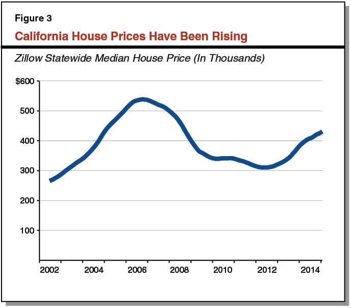
Building Permits Not Responding in Kind. Our main economic scenario—summarized in Figure 1—continues to assume that California residential building permits return over the next several years to levels one would expect based on population growth and historical household formation trends. Yet, it is possible that residential building will not return to these levels or will take much longer to do so than we have assumed. Data suggests that the number of household formations—for example, when younger people move out of parents’ homes—has fallen considerably. There are several possible explanations for this trend. One is that first–time homebuyers are finding it more difficult to purchase homes at current prices. It is also possible that, despite strong demand and rising prices, various factors are preventing developers from increasing production of new housing. These factors may include heightened caution among developers and local government resistance to additional building. Alternatively, Californians may be altering fundamentally their economic, lifestyle, and related choices concerning homes. If these trends continue, they could result in meaningful changes in the California economy—some negative and some positive—affecting construction employment, sales taxes, property taxes, income taxes, population growth, and housing affordability. Our office anticipates releasing additional analyses of issues concerning housing supply, demand, and prices in publications over the next year or so. It is possible that future outlooks concerning California’s housing market will be quite different from the one in this publication.

State General Fund Revenues

Figure 4 summarizes state General Fund revenues and transfers under our main economic scenario. Figure 5 compares this revenue outlook to ones that our office and the administration released in May 2014 for 2013–14 and 2014–15. (The administration’s May revenue outlook was used by the Governor and the Legislature as the basis for the 2014–15 Budget Act in June 2014.)

As noted above, our November 2014 main scenario reflects (1) our best estimate, as of now, of near–term economic conditions and (2) an assumption that growth generally will continue—and in some respects, accelerate—over the next few years. Actual results will vary from our current revenue outlook, either positively or negatively (and perhaps by billions of dollars), particularly in the later fiscal years displayed.

Rainy–Day Fund Transfers Reflected in Revenue Tables. Consistent with the administration’s method of displaying the state’s fiscal condition, Figures 4 and 5 and other tables in this publication deduct transfers from the General Fund to the state’s rainy–day accounts, displaying them as transfers out of the General Fund. These transfers out are listed as negative numbers in Figures 4 and 5, for example. This is a change in practice for our office, such that the numbers in these figures are not directly comparable to those in prior LAO publications. Figure 5 shows the May and November 2014 revenue estimates on an “apples–to–apples” basis in order to improve comparability.

General Fund Revenues Above Budget Act Projections

Both 2013–14 and 2014–15 Appear Above Budget Projections. State revenue collections finished 2013–14 above the projections that were included in the June 2014 state budget act. In 2014–15, monthly revenue collections have also been running over $1 billion above the budget projections, based on preliminary data through the end of October.

As shown in Figure 5, we currently expect total revenues and transfers for 2013–14 to be booked at $92 million above the June 2014 budget projections. For 2013–14, gains for the personal income tax (PIT) and corporation tax (CT) were offset by declines, relative to budget act projections, for the SUT and unclaimed property revenues.

For 2014–15, we currently project revenues and transfers to end the fiscal year about $2 billion above the June 2014 budget projections. For 2014–15, expected gains for PIT, CT, and the state’s insurance tax are being offset by weakness, relative to budget act projections, for the SUT and some minor state revenue sources. We discuss some of the assumptions underlying these figures below.

Personal Income Tax

Dominant Revenue Source. In our main scenario, California’s PIT makes up about two–thirds of state General Fund revenues and transfers for the foreseeable future—both before and after the temporary Proposition 30 rate increases expire for the state’s highest–income PIT filers. As we have noted previously, the end of the Proposition 30 PIT rate increases will not necessarily cause a sudden revenue drop off—a “cliff effect”—for the annual state budget process. Because these rate increases expire at the end of calendar year 2018, it means that state PIT revenues essentially will include an entire fiscal year of Proposition 30 revenues in 2017–18, half a fiscal year of those revenues in 2018–19, and none of the Proposition 30 revenues in 2019–20. Accordingly, if the economy is growing at that time, as our main scenario assumes, then the expiration of Proposition 30 is likely to result in a slowing of PIT revenue growth in 2018–19 and 2019–20, but not an outright decline in PIT revenues.

Recent Strong Growth of Wage and Salary Withholding. Wages and salaries are a large and generally stable part of California’s PIT revenue base. Employers are required to withhold part of each employee’s paycheck each month and send this money to the state to cover the PIT due on the employee’s income. Withholding makes up about two–thirds of net PIT collections each year. The revenue stream from these withholding payments provides a real–time indicator of the growth of wage and salary income.

Withholding growth has been strong in 2014. Withholding for each month from April to October has been between 7 percent and 11 percent above the same month in 2013 (after adjusting for variation in the number of processing days in a given month from one year to the next). For 2014 as a whole, we assume that wages and salaries for California resident PIT filers will be 6.7 percent above 2013 levels—notably higher than the 6 percent growth we projected in May, as well as the 5 percent growth assumed in the June 2014 state budget package. In 2015, our main scenario assumes that wage and salary growth moderates to 5.1 percent.

Estimated Payments Also Showing Strong Growth . . . Taxpayers who have significant income from sources other than wages and salaries are required to make quarterly estimated payments. Sources of such income include capital gains from sales of assets such as stocks and real estate, interest and dividend payments, and profits of businesses that are not subject to the state’s CT. As estimated payments come in each year in April, June, and September, they provide early indications of the total amount of taxable nonwage income that higher–income taxpayers will earn that year. In addition to those estimated payments, other 2014 estimated payments will come into the state treasury in December and January, followed by final or extension payments in April. In many years, high–income taxpayers make large estimated payments in December and January and large payments in April to “settle up” their annual tax liabilities.

For tax year 2014, the first three estimated payments are running about 15 percent above the comparable months in 2013. This is a significant increase, and it contributes to our main scenario assumption that the net amount of capital gains income reported on California residents’ PIT returns in 2014 will be $143 billion—up significantly from the $105 billion assumed for 2014 net capital gains in the June 2014 state budget package.

. . . But Our Outlook Makes Cautious Assumptions About 2014 Capital Gains. Despite our positive outlook for capital gains, relative to the most recent budget act assumptions, we believe that our assumptions for 2014 capital gains—and estimated payments generally—are cautious. We think there is a significant possibility that capital gains reported on 2014 PIT returns will prove to be higher than we now assume. The S&P 500 stock index, for example, has risen substantially in recent months—considerably above our prior expectations. The trend in stock and other asset prices, as well as recent trends in personal income, suggest that 2014 taxable income from capital gains and business activity will be above levels indicated by estimated payments that have been received to date. Our near–term fiscal outlook, however, adopts the cautious assumption that revenue from estimated payments through January 2015 and final payments in April 2015 will be fairly consistent with the estimated payment trend observed to date this year. If capital gains and other estimated payment sources are stronger than we now assume, this could easily increase 2014–15 state PIT revenues by $1 billion or more above our current outlook. As discussed elsewhere in the publication, virtually all of those increased 2014–15 revenues would go to schools and community colleges under the state’s Proposition 98 minimum funding guarantee.

Modest Future Stock Price Growth Assumed. California’s PIT is heavily reliant on high–income taxpayers who pay the highest marginal PIT rates and who receive a large share of capital gains and business income. In fact, the top 1 percent of California PIT filers paid 50 percent of the state’s personal income taxes in 2012. Capital gains—generating over $12 billion of PIT revenues in 2014–15, according to our forecast assumptions—are one major source of year–over–year volatility in PIT collections. As they are closely connected with trends of highly variable stock prices, they are impossible to predict far in advance with any precision. The S&P 500 stock index closed at 2,040 on November 14, 2014—up about 250 points from one year before. In our main scenario, we assume that the S&P 500 stock index retreats somewhat from these strong recent gains by declining to just over 1,925 in early 2015 and remaining flat throughout the rest of 2015. We assume modest growth of about 3 percent per year in the S&P 500 index in our main scenario beginning in 2016. While every forecast of California’s state budget must make assumptions about stock prices—either explicitly or implicitly—actual results will vary from our future assumptions either positively or negatively in any given year. As we discuss in Chapter 5, a large stock market drop—if one were to occur—could cause state revenues to fall by billions of dollars in a single year.

Sales and Use Tax

Below 2014 Budget Projections. Estimated General Fund SUT revenue totaled $22.3 billion in 2013–14, $508 million lower than the amount assumed in the 2014–15 budget. In our main economic scenario, SUT receipts increase by 5.3 percent in each of the next two fiscal years, totaling $23.4 billion in 2014–15 and $24.7 billion in 2015–16. Our 2014–15 estimate is $403 million lower than the assumption in the June 2014 state budget. Under our main scenario, SUT revenues then grow more slowly over the following two fiscal years as the one–quarter cent Proposition 30 SUT increase ends in December 2016. As with the Proposition 30 PIT increases, the timeline of this tax expiration means that the state will see a gradual drop off in Proposition 30 SUT revenues over two fiscal years.

Prior Years’ Local SUT Adjustment. As discussed in Chapter 1, we assume that the General Fund’s entering fund balance in 2013–14 will be lowered by $358 million to reflect a prior–year misallocation of SUT revenues to local governments that recently was identified and corrected by the state. We understand that this amount will be booked in the state’s budgetary accounting system in this way, thereby not affecting any particular fiscal year’s accrued SUT revenues.

Corporation Tax

Above 2014 Budget Projections. Refunds to CT payers have been running below June 2014 budget assumptions. This is a positive development for net CT collections by the state. As a result, in our main scenario, estimates of net CT revenues accrued to 2012–13 and of CT revenues in 2013–14 and 2014–15 are all above budget act projections. In that scenario, we estimate that CT revenue will grow from $8.5 billion in 2013–14 to $9.5 billion in 2014–15 and $10.4 billion in 2015–16. Our near–term CT outlook reflects strong growth in recent CT collections and an assumption that recent trends in CT refunds will continue. Our main scenario assumes that corporate income will continue to grow through 2015. In later years, however, corporate income is assumed to decline somewhat from these high levels.

Operating Loss Deductions Expected to Remain at Elevated Levels. As we anticipated in last year’s Fiscal Outlook, corporations significantly increased their use of net operating loss (NOL) deductions from $3 billion in 2011 to approximately $19 billion in 2012. The use of NOL deductions—in which corporations deduct a prior loss from current tax year profits—was suspended for most corporations during tax years 2008 through 2011. We anticipate that NOLs will remain at elevated levels throughout the forecast period, but NOL use in any given year is highly uncertain. We also expect use of the state’s largest corporate tax credit program, the research and development tax credit, to increase somewhat in future years. Beginning in the 2016 tax year, our forecast takes into account recent legislative actions to increase the amount of credits available under the film and television tax credit and California Competes tax program.

Other Issues

Unclaimed Property Revenues Lower Than June 2014 Budget Projections. The State Controller’s Office receives various types of property considered to be abandoned by owners. The state maintains an obligation to reunite these properties with their rightful owners, should they make a claim. Each month, however, amounts unclaimed in excess of $50,000 become General Fund revenues. June and July are the most important cash months for unclaimed property. Official reports for July 2014 show cash receipts well below 2014–15 budget assumptions. We assume this reflects an ongoing reduction in the amount of property received by the state, affecting each year starting with 2013–14. Over 2013–14 and 2014–15 combined, we estimate that revenues related to unclaimed property will be over $100 million lower than assumed in the 2014–15 budget package. Because various parts of the program expire after 2015–16 under current law, we expect these revenues to decrease around 10 percent in 2016–17 and remain steady thereafter.

$1.3 Billion in Special Fund Loans Assumed Repaid in 2015–16. Figure 6 displays the loans we assume that the General Fund will repay to various state special funds in 2015–16. (If all of those payments were made, $1.8 billion in special fund loans would remain outstanding.) We assume that any loan with a deadline in law will be repaid by that date. In addition, when it appears a special fund requires a loan repayment, we assume any loan outstanding to that fund is repaid. As discussed in Chapter 1, special fund loan repayments count toward the debt payment requirements of Proposition 2.

The three largest loan repayments shown in Figure 6 have 2015–16 deadlines in law. It appears to us that the Legislature may have considerable flexibility in determining whether to repay these loans. In addition, while the Greenhouse Gas Reduction Fund loan does not have a deadline in current law, the 2014–15 budget package authorized amounts to be repaid and used for the high–speed rail project beginning in 2015–16. Of the $400 million balance currently outstanding from that fund, we assume that half is repaid in 2015–16 and that the remainder is repaid in 2016–17.

Major Penalty and Fine Revenue Uncertain. Each year, the state General Fund receives payments from court and administrative judgments. In 2012–13, for example, $23 million of such payments were received by the General Fund. The June 2014–15 budget assumed that the state would receive $323 million of such payments in 2014–15, including a potential $300 million payment from the Pacific Gas and Electric (PG&E) Company, the possibility of which had been disclosed publicly to PG&E investors earlier in the spring. The penalties and fines were related to PG&E operations and practices, including the 2010 rupture of a gas pipeline in San Bruno. On September 2, the California Public Utilities Commission issued decisions by administrative law judges that sought to impose a $1.4 billion penalty on PG&E, including a $950 million payment to the state General Fund. On October 2, PG&E filed appeals concerning these decisions. Accordingly, there is now uncertainty about the timing of any General Fund payments by PG&E, as well as the amounts of those payments. Due to this uncertainty, we assume no General Fund payments by PG&E in our revenue outlook. It is quite possible that some PG&E payments will be received by the General Fund in the future, and if so these payments would improve the budget’s bottom line.

Chapter 3: Spending Outlook

Figure 1 displays our estimates of General Fund spending for 2013–14 and 2014–15, as well as our outlook for spending through 2019–20. The estimates in Figure 1 reflect our main economic scenario. Assuming continued moderate economic growth, we estimate General Fund spending to grow at an average annual rate of 2.4 percent. This slow growth rate is primarily explained by key assumptions concerning Proposition 98. The assumed expiration of Proposition 30’s taxes and our assumption that capital gains revenues decline contribute to slow growth in the Proposition 98 minimum guarantee in the later years of the outlook. Further, our General Fund spending outlook is affected by local revenues because Proposition 98 is funded by a combination of state General Fund and local property taxes. While we project growth in overall Proposition 98 funding, our strong outlook for local property tax growth offsets what would otherwise be higher General Fund spending necessary to meet Proposition 98 requirements. Because Proposition 98 General Fund spending represents around 40 percent of the budget, these assumptions are key factors in the slow growth rate of spending overall. We discuss this and other spending trends throughout this chapter. In general, this chapter discusses our main scenario spending outlook unless noted otherwise.

Education

Education Outlook. Below, we discuss our outlook for Proposition 98, the universities, and the state’s financial aid programs. Our Proposition 98 outlook estimates spending for preschool, elementary and secondary education (commonly referred to as K–12 education), and the California Community Colleges (CCC) combined. Our university outlook estimates spending for the California State University (CSU), the University of California (UC), and Hastings College of the Law (Hastings). Our student financial aid outlook estimates spending for the Cal Grant program, Middle Class Scholarships, and a few small specialized programs.

Proposition 98

Proposition 98 Minimum Guarantee for Schools and Community Colleges. State budgeting for schools and community colleges is governed largely by Proposition 98, passed by voters in 1988. The measure, modified by Proposition 111 in 1990, establishes a minimum funding requirement, commonly referred to as the minimum guarantee. Both state General Fund (including Education Protection Account) and local property tax revenue apply toward meeting the minimum guarantee. In addition to Proposition 98 funding, schools and community colleges receive funding from the federal government, other state sources (such as the lottery), and various local sources (such as parcel taxes).

Calculating the Minimum Funding Guarantee. The Proposition 98 minimum guarantee is determined by one of three tests set forth in the State Constitution (see Figure 2). These tests are based on several inputs, including changes in K–12 average daily attendance (ADA), per capita personal income, and per capita General Fund revenue. Though the calculation of the minimum guarantee is formula–driven, a supermajority of the Legislature can vote to suspend the formulas and provide less funding than the formulas require. This happened in 2004–05 and 2010–11. In some cases, including as a result of a suspension, the state creates an outyear obligation referred to as a “maintenance factor.” The state is required to make maintenance factor payments when year–to–year growth in state General Fund revenue is relatively strong. Though in most years the state has provided an amount at or close to the minimum guarantee, the state has discretion to provide any amount above the minimum guarantee.

2013–14 and 2014–15 Updates

2013–14 Minimum Guarantee Up Slightly From Budget Act Estimates. Figure 3 compares our updated estimates of the 2013–14 minimum guarantee with what was assumed in the most recently enacted spending plan. Our estimate of the 2013–14 minimum guarantee is up $177 million. Of this amount, $100 million is associated with an upward revision in K–12 ADA. Latest ADA estimates are up about 10,000 ADA (0.17 percent) from budget act estimates. The remainder of the increase is due to 2013–14 General Fund revenue being higher than budget act assumptions. General Fund revenue that counts toward Proposition 98 is up $137 million, with the corresponding increase in the guarantee slightly more than half this amount. Test 3 remains the operative test for calculating the 2013–14 guarantee. Given the increase in the guarantee, the size of the new maintenance factor created is smaller compared to budget act assumptions ($381 million, down from $458 million).

2013–14 General Fund Proposition 98 Costs Up Slightly. Though the guarantee is up $177 million, the General Fund share of the guarantee is up only $63 million. This is because our estimate of local property tax revenue also is up from budget act estimates. Local property tax estimates are up a net of $114 million due to various adjustments (some offsetting), including slight changes in regular and supplemental property tax payments as well as updated estimates of revenue shifted to school and community college districts from former redevelopment agencies (RDAs).

2014–15 Minimum Guarantee Up $2.3 Billion From Budget Act Estimates. Figure 3 also compares our updated estimates of the 2014–15 minimum guarantee with what was assumed in the 2014–15 Budget Act. The increase in the 2014–15 guarantee is due primarily to General Fund revenue being higher than budget assumptions. General Fund revenue that counts toward Proposition 98 is up $2.2 billion, yielding a near dollar–for–dollar increase in the guarantee. Test 1 remains the operative test for calculating the 2014–15 guarantee. Given the significant increase in General Fund revenue, the size of the required maintenance factor payment is up notably (now estimated at $3.8 billion, up from the budget act estimate of $2.6 billion). As of the end of 2014–15, we estimate the state’s total outstanding maintenance factor obligation to be $2.7 billion.

2014–15 General Fund Proposition 98 Costs Up Significantly. Of the $2.3 billion increase in the guarantee, the General Fund share increases $2.1 billion and the local property tax share increases $259 million. Similar to 2013–14, the increase in local property tax revenue is due to various relatively minor adjustments.

Increase Sufficient to Trigger Paydown of All Remaining Education Deferrals. Chapter 32, Statutes of 2014 (SB 858, Committee on Budget and Fiscal Review), set forth that if the minimum guarantees for 2013–14 or 2014–15 came in higher than budget act assumptions, the first $992 million in higher–than–assumed growth would be used for paying down remaining education deferrals. We estimate the 2013–14 and 2014–15 minimum guarantees are up a combined $2.5 billion—high enough to trigger the paydown of all remaining deferrals by the end of 2014–15.

$1.5 Billion Available for Other One–Time Purposes. After retiring all education payment deferrals, $1.5 billion would remain available under our forecast for additional Proposition 98 spending in 2014–15. Given the 2014–15 school year is underway, this funding in practical terms is available for one–time purposes. In recent years, the state has prioritized various one–time purposes, including paying down the education mandate backlog, paying down outstanding Emergency Repair Program (ERP) obligations, and supporting new initiatives, such as implementation of the Common Core State Standards and creation of the California Career Pathways Trust. We estimate the state currently has a total of $4.3 billion in unpaid education mandate claims ($3.9 billion for schools and $405 million for community colleges). It has $274 million in outstanding ERP obligations.

Temporary Revenue Surge Would Increase 2014–15 Guarantee. The minimum guarantee in 2014–15 is highly sensitive to changes in General Fund revenue. This is because the state has a large outstanding maintenance factor obligation, Test 1 is operative, and the state has chosen to make maintenance factor payments on top of the Test 1 level. In this situation, the guarantee increases virtually dollar–for–dollar with growth in General Fund revenue. Because of this heightened sensitivity to changes in General Fund revenue, together with the possibility that personal in come tax (PIT) revenue could be higher in 2014–15 than assumed in our main forecast scenario, one of the economic scenarios we considered involved a hypothetical, temporary surge of capital gains revenue in 2014–15. Under this surge scenario, we assume General Fund revenue is above our main scenario by $1.5 billion in 2014–15 and $0.5 billion in 2015–16. The $1.5 billion General Fund increase in 2014–15 results in a $1.5 billion increase in the 2014–15 minimum guarantee. Because the guarantee in 2015–16 builds upon the amount provided the prior year, it too increases by $1.5 billion. Under this scenario, the “bottom line” of the General Fund benefits virtually none from the revenue growth in 2014–15 and is worse off moving forward. (We discuss the temporary revenue surge scenario’s effects on the state budget in more detail in Chapter 5.)

If General Fund revenue in 2014–15 ends up more than $1.6 billion above our main outlook, then the spike protection provisions of the Constitution become operative. As a result, any growth in the guarantee above $1.6 billion in 2014–15 would be excluded from the Proposition 98 calculations in 2015–16. This reduces the 2015–16 guarantee from what it would be otherwise, thereby limiting potential fiscal effects on the rest of the state budget.

2015–16 Budget Planning

2015–16 Guarantee $2.6 Billion Higher Than Updated 2014–15 Guarantee. Under our main scenario (see Figure 4), the minimum guarantee grows from $63.2 billion in 2014–15 to $65.8 billion in 2015–16—an increase of $2.6 billion (4.1 percent). Test 2 is operative, with the increase in the guarantee driven by growth in per capita personal income. We assume K–12 ADA declines by 0.4 percent, but the decline does not affect the guarantee. This is because the Constitution has a two–year hold harmless provision that insulates the guarantee from initial drops in K–12 ADA. (As we assume drops in K–12 ADA every year of the forecast period, the guarantee under our forecast would be affected beginning in 2016–17.) The state would not be required to make a maintenance factor payment in 2015–16 (as the Test 2 and Test 3 levels are very close, with growth in per capita personal income similar to growth in General Fund revenue).

Entire Increase in Guarantee Covered by Higher Local Property Tax Revenue. Under our main scenario, General Fund Proposition 98 costs drop slightly in 2015–16 despite the increase in the guarantee. This is because local property tax revenue is $2.7 billion (16 percent) higher in 2015–16 compared to 2014–15. The large increase in property tax revenue is mainly a result of the following three factors. (The increases identified below are offset by a small reduction in various other components of our property tax estimate.)

• “Triple Flip” Ends. The largest factor is the end of the triple flip. Under the triple flip, the state (1) diverted local sales tax revenue to pay off the state’s Economic Recovery Bonds (approved by voters in 2004 to help close the state budget gap), (2) backfilled cities and counties with school and community college property tax revenue, and (3) backfilled schools and community colleges with state General Fund. Under our main forecast, the state retires the Economic Recovery Bonds by the end of 2014–15. As a consequence, $1.7 billion in local property tax revenue flows back to schools and community colleges in 2015–16.
• Underlying Property Tax Revenue Grows at Healthy Rate. Under our main scenario, we project underlying property tax revenue to increase 5.5 percent in 2015–16. This is slightly lower than the prior–year growth rate (6.1 percent) but still healthy by historic standards. The 5.5 percent increase equates to $950 million in additional local property tax revenue.
• Revenue Shifts From Former RDAs Continue to Increase. We project that ongoing property tax revenue shifted from RDAs to schools and community colleges increases about $200 million from 2014–15 to 2015–16—growing to about $1 billion in 2015–16. (We project one–time shifts relating to former RDA assets will remain roughly flat in 2015–16 before decreasing steadily through the end of the forecast period.)

$6.4 Billion Available for Proposition 98 Priorities. Figure 5 identifies the amount of funding available for Proposition 98 priorities in 2015–16 under our main scenario. With a projected 2015–16 minimum guarantee of $65.8 billion and an ongoing Proposition 98 spending level currently at $59.4 billion, the state has $6.4 billion for its 2015–16 Proposition 98 priorities. The Legislature’s key Proposition 98 decisions in the coming budget cycle likely will revolve around how best to allocate these funds among preschools, schools, and community colleges; how much to designate for ongoing versus one–time purposes; and how much to use for starting new initiatives versus sustaining or extending existing efforts.

In Hypothetical Economic Slowdown, Guarantee Could Decline. Because the outlook for the minimum guarantee in 2016–17 can help inform the Legislature’s 2015–16 decisions, we also examined a hypothetical economic slowdown scenario that is more pessimistic than our main scenario (see Figure 4). In this slowdown scenario, we assume General Fund revenue is below our main forecast by $2.6 billion in 2015–16 and $8.2 billion in 2016–17. (As discussed in more detail in Chapter 5, this would reflect a moderate slowdown in overall economic activity and a sharp stock market decline in 2016.) Despite the drop in General Fund revenue, the minimum guarantee in 2015–16 is largely unaffected. Under this scenario, the operative test shifts from Test 2 to Test 3, but a supplemental appropriation is triggered under Test 3 that results in bringing the guarantee almost back up to the Test 2 level. The Test 3 supplemental appropriation is set forth in statute. It is intended to ensure that the Proposition 98 and non–Proposition 98 sides of the budget are treated similarly in tight fiscal times. Though the 2015–16 guarantee is largely unaffected, the 2016–17 guarantee under the slowdown scenario drops $700 million from 2015–16. Under the slowdown scenario, if the Legislature had committed all available Proposition 98 funds in 2015–16 for ongoing purposes, it would face pressure in 2016–17 either to reduce ongoing programs or raise additional revenue to sustain the prior–year ongoing funding level.

Designating Funds for One–Time Purposes Would Minimize Outyear Risks. Given the volatility of the state’s General Fund revenues, our main scenario realistically could under– or over–estimate the minimum guarantee by billions of dollars. If the 2014–15 through 2016–17 guarantees are higher than under our main scenario, the state likely could make greater progress in implementing the Local Control Funding Formula (LCFF). Alternatively, if the guarantee over this near–term period is lower than in our main scenario, the state likely would face difficulty sustaining ongoing Proposition 98 (and non–Proposition 98) programs. Because of the possibility that the guarantee in future years could be lower than the 2015–16 guarantee, we recommend the Legislature designate some Proposition 98 funds in 2015–16 for one–time purposes. Doing so would mitigate downsize risk while also helping the state pay down its outstanding one–time obligations (most notably, the multibillion dollar education mandates backlog).

Outlook for Later Years

Though both the Legislature and schools likely view near–term Proposition 98 issues as the most pressing, they face several significant issues throughout the forecast period. Most notably, the phase out of Proposition 30 taxes, the phase in of LCFF funding increases, and the cost pressure related to the phase in of the California State Teachers’ Retirement System (CalSTRS) rate increases, all unfold throughout this period. Additionally we examine whether a Proposition 2 deposit, with the accompanying triggered reductions in school district reserve levels, might happen sometime during the period. Below, we first describe Proposition 98 under our main scenario through 2019–20 and then discuss each of the above issues in more detail.

In Main Scenario, Guarantee in 2019–20 More Than $11 Billion Higher Than in 2014–15. Figure 6 shows our main Proposition 98 scenario for 2014–15 through 2019–20. Under our main scenario, the minimum guarantee grows from $63.2 billion in 2014–15 to $74.5 billion in 2019–20—an average annual growth rate of 3.3 percent. General Fund Proposition 98 costs grow more slowly—from $46.5 billion in 2014–15 to $49.9 billion the last year of the period. This slow growth in General Fund costs results from the relatively fast growth in local property tax revenue, which increases from $16.7 billion in 2014–15 to $24.6 billion the last year of the period. The average annual growth over the period is 1.4 percent for the General Fund and 8.1 percent for local property tax revenue.

Local Property Tax Revenue Assumed to Grow at About Historical Average. Following the end of the triple flip, we assume local property tax revenue continues to increase steadily over the period. Under our main scenario, assessed property values grow at about 6 percent each year over the 2016–17 through 2019–20 period—similar to the historical average. This corresponds to growth of about $1 billion per year. In addition, under our main scenario, RDA residual revenue increases by slightly more than $200 million per year. When combined with several other smaller revenue components, total school and community college local property tax revenue increases, on average, $1.3 billion each year of the period.

Slower Growth in Guarantee as Proposition 30 Revenues Phase Out. Under our main scenario, the growth rates in the guarantee during the first part of the period are stronger than during the latter part of the period. For example, the guarantee grows 4.1 percent in 2015–16 and 2.5 percent in 2019–20. The smaller growth rates throughout the latter part of the period are due in part to the phase out of Proposition 30 revenues, with the sales tax rate increases phasing out over 2016–17 and 2017–18 and the PIT rate increases phasing out over 2018–19 and 2019–20. Because the tax increases phase out gradually over four fiscal years, the effect on the guarantee is lessened. The slower growth rates, however, would make funding ongoing program expansions more difficult.

State Could Make Progress but Likely Not Fully Implement LCFF by 2019–20. In 2013–14, the state replaced most of its former school funding formulas with the LCFF. In creating the LCFF, the state set funding targets considerably higher than the 2012–13 funding levels and specified that the targets were to be adjusted annually for cost–of–living adjustment (COLA). Given the higher funding targets, the state expected the LCFF would not be fully funded until 2019–20. For 2014–15, we estimate the LCFF is 80 percent funded. Under our main scenario, the LCFF would be 91 percent funded by 2019–20 if the state dedicated the increase largely to LCFF. (Our estimate assumes the state creates no new categorical programs throughout the period and all existing categorical programs but adult education receive only ADA growth and COLA. Consistent with statutory intent, we assume the adult education program receives an additional $500 million in 2015–16. We also assume community colleges continue to receive roughly 11 percent of Proposition 98 funds.) Given the higher LCFF targets, growth in the minimum guarantee would have to outpace COLA rates significantly to fully fund the LCFF by the end of the forecast period. Whereas annual COLA rates range from 1.6 percent to 2.9 percent over the 2015–16 through 2019–20 period, annual growth in the guarantee ranges from 2.5 percent to 4.1 percent—somewhat but not markedly higher than the COLA rates.

CalSTRS Rate Increases Also Phasing in Over Period. Based upon legislation adopted in 2014 that is designed to address outstanding CalSTRS’ liabilities, school and community college districts’ contribution rates are set to increase beginning in 2014–15 and every year thereafter of the forecast period. In 2014–15, the rate increase is 0.63 percent (for a total district contribution rate of 8.88 percent). By the last year of the forecast period, the total cumulative rate increase is 9.88 percent (for a total district contribution rate of 18.13 percent). CalSTRS estimates that districts’ contribution costs will be $3.1 billion higher in 2019–20 compared to 2014–15. Under our main scenario, the minimum guarantee in 2019–20 is $11.3 billion higher than 2014–15.

No Deposit Into Public School System Stabilization Account (PSSSA) Projected. Proposition 2, approved by voters in November 2014, created a new reserve—the PSSSA. Proposition 2 is connected with a recently enacted state law that triggers a reduction in school district reserve levels the year after the state makes a deposit into the PSSSA. Under our main scenario (as well as our surge and slowdown scenarios), the state would not make a deposit into the PSSSA. The cap on school district reserve levels therefore would not be triggered at any time during the forecast period.

Universities

The state’s public universities consist of CSU, UC, and Hastings. The CSU educates about 430,000 undergraduate and graduate students at 23 campuses. The UC educates about 240,000 undergraduate and graduate students at ten campuses, and Hastings educates about 1,100 graduate students in law at its one campus. The universities receive support for their core instructional programs from a combination of state funds and student tuition revenue.

Considerable Discretion in University Budgeting. In building CSU’s and UC’s budgets, the Legislature is constrained by few constitutional requirements and few federal requirements—notably fewer than for many other areas of the state budget. Greater discretion also stems from the ability of CSU and UC to raise revenue through student tuition increases. For forecasting purposes, this high level of discretion translates into university spending being very sensitive to future legislative and tuition decisions.

Forecasting Current–Law Provisions Not Necessarily Most Helpful Approach. Additionally, the state over the last few years has tended not to adhere closely to certain statutory and Master Plan provisions affecting CSU’s and UC’s budgets. The state lacks guiding policy altogether for other university budget areas. Below, we highlight the major areas for which current law provides little guidance in developing forecasting assumptions.

• COLA. Statute specifies the universities are not to receive automatic COLAs. The state, however, has provided CSU and UC with base increases the last two years.
• Eligibility Pools and Enrollment Growth. Whereas the Master Plan sets forth that CSU and UC are to draw from specified high school eligibility pools (the top one–third for CSU and top one–eighth for UC), the state has not undertaken an eligibility study since 2007. As a result, the effect of CSU’s and UC’s recent admission decisions on eligibility is unknown and estimating the need for future enrollment growth has increasingly become guesswork.
• Tuition Levels. Statute sets forth no policy regarding resident tuition levels. The Governor has indicated he would like CSU and UC to freeze resident tuition levels at least through 2016–17. The universities’ tuition levels for undergraduates and most graduate students have been flat for the last four years (since 2011–12). The UC has indicated in its proposed budget that it plans to raise tuition levels up to 5 percent annually for the next five years, beginning in 2015–16. The CSU Trustees have not taken similar action for 2015–16. Whether CSU plans to hold tuition levels flat throughout the entire forecast period remains uncertain.

LAO Outlook for Universities Based Primarily on Current Practice. Rather than a current–law forecast, we assume university spending over the next few years will grow similarly to how it has grown in recent years. Specifically, we assume CSU and UC will (1) continue to receive base increases; (2) fund any enrollment growth, faculty compensation increases, and most increases in debt–service costs from within those base increases; and (3) hold tuition levels flat. For 2015–16 (and the remainder of the forecast period), we assume annual base increases of 4 percent. Consistent with practice over the last two years, we link these increases to UC’s base budget such that the projected dollar increase is the same for CSU and UC each year. For 2015–16 and 2016–17, we assume CSU receives additional funding beyond its base increase to cover projected increases in its lease–revenue debt service, consistent with legislative action taken in 2014–15.

Under LAO Outlook, University Spending Grows by $243 Million in 2015–16. Of this amount, $127 million is higher CSU spending and $116 million is higher UC spending. The increase grows to a total of $256 million in 2016–17, reaching $280 million by the last year of the forecast period. As noted earlier, the Legislature has considerable discretion in funding the universities and could choose to provide more or less than these amounts. Annual funding increases also could be affected by tuition increases. Revenue raised from tuition increases could offset part of the General Fund augmentations. Given final tuition levels for 2015–16 and the rest of the period are uncertain, the universities’ total increases in core funding could differ significantly from the amounts shown under our outlook.

Assumed Spending Level Under LAO Outlook Roughly Equates to COLA in Core Funding. Roughly half of CSU’s and UC’s core funding comes from the state General Fund. Thus, a 4 percent base General Fund increase roughly equates to a 2 percent increase in core funding. This is about the same as the projected 2015–16 U.S. state and local price deflator (2.2 percent). Demographically, California’s traditional college–age population (18–24 years of age) is projected to decline 1.2 percent in 2015. High school graduates also are projected to decrease slightly in 2015–16, though transfers from community colleges could increase slightly due to increases in community college enrollment as well as improvements in transfer pathways (particularly from CCC to CSU). If the universities were to hold enrollment levels flat given these demographic trends, their 2015–16 per–student funding levels would remain about the same in real terms as in 2014–15.

Financial Aid

The California Student Aid Commission (CSAC) is responsible for administering state financial aid programs. The state’s largest aid program is the Cal Grant program, which serves about 316,000 undergraduate students. This program currently is funded with a combination of state General Fund and federal Temporary Assistance for Needy Families (TANF) monies.

Outlook for Student Financial Aid Based Primarily on Current–Law Provisions. Our outlook assumes continued implementation of existing statutory financial aid policies. Specifically, we assume continued phase–in of the Middle Class Scholarship program, Cal Grant awards for Dream Act students, and scheduled Cal Grant award reductions for students attending nonprofit colleges.

Other Key Cal Grant Assumptions. We assume continued growth in Cal Grant participation based on historical trends and ongoing efforts to increase the number of high school students applying for financial aid. Specifically, we assume 3 percent annual participation growth throughout the forecast period. Legislation adopted in 2014 requiring high schools to submit student grades to CSAC electronically will contribute to this growth. Consistent with our CSU and UC forecasts, we assume no tuition increases and no enrollment growth at the universities. We also assume the state continues to use federal TANF funds to offset a portion of General Fund Cal Grant costs.

Under LAO Outlook, Net General Fund Cal Grant Costs Increase by $67 Million in 2015–16. We estimate General Fund costs for Cal Grants will increase by $89 million, offset by $22 million in General Fund savings resulting from scheduled reductions in private college award amounts. Of the cost increases, $53.6 million is participation growth, $29.6 million is continued phase–in of Dream Act awards, and $6 million backfills one–time funding from loan program balances. Cal Grant costs are projected to grow by a net of $79 million in 2016–17. Annual increases slow following full phase–in of the Dream Act in 2016–17, with an increase of $64 million the last year of the forecast period. We project total Cal Grant costs to grow from $1.8 billion in 2014–15 to $2.2 billion the last year of the period.

Too Soon to Forecast Impact of New Tax Credit on Cal Grant Spending. In the 2014 session, the state enacted legislation creating the College Access Tax Credit Fund (College Access Fund). As set forth in the legislation, individuals may make charitable contributions to the College Access Fund and, in turn, receive a large tax credit (starting at $0.60 per $1 the first year, declining to $0.50 per $1 the third year, capped at a total of $500 million statewide). The tax credit sunsets December 1, 2017. Contributions to the fund will support increases in the Cal Grant B access award, which helps low–income students cover non–tuition expenses (such as books, supplies, rent, and transportation). The award amount currently is $1,648 per year. After covering associated tax credit and administrative costs, monies in the College Access Fund will increase the Cal Grant B access award amount. Given the first contributions to the fund only now are being made, we did not forecast contributions to the College Access Fund and the resulting increase in access award amounts. The new fund, however, could result in higher Cal Grant B spending, beginning in 2015–16.

Middle Class Scholarship Spending Increases Next Few Years but Likely by Less Than Initially Planned. The estimated first–year cost of the Middle Class Scholarship program is lower than budgeted, totaling about $70 million (compared with the $107 million appropriation). Campuses report discovering that many potential Middle Class Scholarship recipients already receive sufficient aid to cover at least 40 percent of their tuition and thus are not eligible for awards. In addition, they believe a number of students might not have applied for financial aid in the first year of program implementation because they were unaware they could qualify for scholarships. We estimate Middle Class Scholarship Program costs will grow to $111 million, $173 million, and $237 million in 2015–16, 2016–17, and 2017–18, respectively. Following full phase–in of awards in 2017–18, we estimate costs will grow more slowly—to a total of $244 million at the end of the forecast period (compared with the $305 million ongoing appropriation cap).

Key Policy Decisions Could Increase Financial Aid Costs Significantly. The financial aid outlook is sensitive to changes in higher education enrollment as well as CSU and UC tuition levels. We estimate a 2 percent increase in enrollment at CSU and UC would add about $30 million to Cal Grant costs and $2 million to Middle Class Scholarship costs in 2015–16. We estimate a 5 percent increase in tuition at CSU and UC would increase Cal Grant costs by about $65 million and Middle Class Scholarship costs by $5 million. Altogether, these changes would add about $100 million to financial aid costs in the budget year. In addition, increased participation in financial aid programs resulting from new outreach efforts within CSU and UC (for Middle Class Scholarships) and within high schools (for all aid programs) could raise aid costs by several tens of millions of dollars. Any current–year growth in aid spending not yet reported by CSAC also would have outyear effects.

Health and Human Services

Overview of Health Services Provided. California’s major health programs provide health coverage and additional services for various groups of eligible persons—primarily poor families and children as well as seniors and persons with disabilities. The federal Medicaid program, known as Medi–Cal in California, is the largest state health program both in terms of funding and number of persons served. Beginning January 2014, the Medi–Cal population has grown substantially, reflecting an expansion of those eligible for Medi–Cal and a streamlining of eligibility requirements under the Patient Protection and Affordable Care Act (ACA), also known as federal health care reform. In addition, the state supports various public health programs. Although state departments oversee the management of these programs, the actual delivery of many services is carried out by counties and other local entities. Health programs are largely federally and state funded.

Overview of Human Services Provided. The state provides a variety of human services and benefits to its citizens. These include income maintenance for the aged, blind, or disabled; cash assistance and welfare–to–work services for low–income families with children; protection of children from abuse and neglect; the provision of home–care workers who assist the aged and disabled in remaining in their own homes; and community services and state–operated facilities for the mentally ill and developmentally disabled. Although state departments oversee the management of these programs, the actual delivery of many services is carried out by county welfare and child support offices, and other local entities. Most human services programs have a mixture of federal, state, and county funding.

Overall Spending Trends. The 2014–15 budget provided $29.5 billion in General Fund spending for health and human services (HHS) programs. We now estimate that these General Fund costs in 2014–15 will be slightly higher—by a net of $47 million—in part reflecting higher caseloads than assumed by the budget for certain segments of the Medi–Cal population and for the California Work Opportunity and Responsibility to Kids (CalWORKs) population. Based on current law requirements, we project that General Fund spending for HHS programs will increase to $29.7 billion in 2015–16 and $30.6 billion in 2016–17. This relatively modest growth in General Fund spending over these years is not primarily due to a slowing down in program growth, but rather is largely reflective of changes in how programs are funded. For example, over these years, there is an increase in General Fund savings in Medi–Cal associated with enhanced federal matching funds for the Children’s Health Insurance Program (CHIP) under ACA. In addition, over these years, more General Fund spending in CalWORKs is being offset with county realignment revenues. We assume that spending for HHS programs will eventually reach $34.3 billion in 2019–20 in our main scenario. The bulk of the spending growth in the later years of the outlook reflect increases in caseload for some categories of enrollees and the per–person cost of providing health care services in Medi–Cal. Medi–Cal General Fund spending grows faster in the latter part of the forecast period as savings that offset Medi–Cal General Fund costs in the earlier years are reduced and as the state’s share of costs for the Medi–Cal expansion under federal health care reform ramp up.

Although the average projected annual increase in HHS spending from 2014–15 through 2019–20 is 3 percent, there is substantial variation in spending growth rates by program. For example, over these years, General Fund spending growth for Medi–Cal averages 4 percent per year, while the Supplemental Security Income/State Supplementary Program (SSI/SSP) is projected to have average annual growth of 1.4 percent. General Fund spending for the CalWORKs program is projected to decline at an average annual rate of 10.5 percent, reflecting both projected caseload declines as well as the infusion of non–General Fund funding sources to support the program, as discussed further below.

Anticipated Lower Caseload Growth in Some Programs Relative to Recessionary Years Reduces Cost Pressures. The recession in the latter part of the 2000s raised unemployment and reduced income, resulting in historically high numbers of Californians enrolling in certain state HHS programs. As a result, caseload growth for several HHS programs from 2007–08 (the beginning of the recession) to 2011–12 (post–recession) was well above historical trends. Our main economic scenario assumes moderate employment growth over the next five years. Accordingly, our caseload projections for several HHS programs reflect substantially lower growth rates compared to the experience of the recent recessionary years, and in some cases—such as CalWORKs—we are anticipating caseload declines under our main scenario over some or all of the forecast period. This in turn reduces cost pressures. Below, we discuss spending trends in the major HHS programs.

Medi–Cal

Overall Spending Trends. We estimate that 2014–15 General Fund spending for Medi–Cal local assistance administered by the Department of Health Care Services (DHCS) will be $17.2 billion—approximately 0.2 percent lower than what was assumed in the 2014–15 Budget Act. The slightly lower 2014–15 spending estimate mainly reflects increased savings from the managed care organization (MCO) tax, due to higher–than–predicted caseload for newly eligible populations under the ACA. (This is known as optional expansion.) Our 2014–15 estimate also reflects higher caseload but lower per–enrollee fee–for–service (FFS) costs associated with recent Medi–Cal enrollment among previously eligible populations who, absent the ACA, would not have enrolled in Medi–Cal. (This is known as the mandatory expansion.) Under our main scenario, General Fund support decreases 1.1 percent to $17.1 billion in 2015–16 and then grows to $17.9 billion in 2016–17—a year–over–year increase of 4.8 percent. General Fund costs are projected to decrease in 2015–16 largely as a result of savings associated with increased federal funding of CHIP under ACA (discussed in more detail below), which offsets other increases in program costs. The growth in General Fund spending in 2016–17 compared to 2015–16 is mainly a function of underlying program growth and decreased savings associated with the MCO tax (discussed in more detail below).

Future Changes in Caseload. Medi–Cal has experienced major caseload growth since the January 1, 2014 implementation of key provisions of the ACA. For September 2014, the preliminary count of enrollees—which will likely be revised upward to include individuals later found to be retroactively eligible—was over 11 million. This preliminary count includes 2 million individuals who became newly eligible for Medi–Cal under the optional ACA expansion and 1.1 million previously eligible individuals who enrolled as part of the mandatory expansion.

While the main effect of the mandatory and optional expansions is mostly a one–time caseload increase in the present and short–run, we also expect changes in the state’s economy and population to influence the longer–run trend for enrollment growth (or decline) in the program. This is based on our analysis of historical patterns in caseload over the past decade. For example, enrollment among the families and children population grew nearly 11 percent during the recession. However, it grew only 1 percent annually between 2011 and 2013. As discussed below, we expect these growth rates to further level off as families’ incomes rise with the improving economy.

Our outlook addresses movements in caseload due to both (1) the immediate influx from the mandatory and optional ACA expansions and (2) the longer–run historical relationship between Medi–Cal enrollment and the state’s economic conditions and demographic trends. We project that by 2015–16, the average monthly enrollment associated with ACA expansions will stabilize at around 2.1 million for the optional expansion and 1.1 million for the mandatory expansion. Under our main economic scenario, we project that by 2016–17, the underlying trend for enrollment among families and newly eligible adults will switch to a slight decrease of less than 1 percent annually. This translates to about 8,000 fewer enrollees per year. Caseloads for seniors and persons with disabilities historically track the state’s demographics rather than economic factors. We estimate enrollment among seniors will grow by about 2 percent in both 2015–16 and 2016–17, while enrollment among persons with disabilities will grow by 3 percent in both years. This adds about 25,000 enrollees per year to each category.

Growth in FFS and Managed Care Expenditures. Growth in Medi–Cal expenditures is related to growth in costs across the broader health care sector. For example, each year the state’s actuary certifies the capitated rates paid to Medi–Cal managed care plans. As part of the rate development process, the actuary incorporates information and assumptions about future health care cost trends, including medical inflation. We assume these types of relationships between Medi–Cal expenditures and broader health care costs will continue to hold throughout the forecast period. Based on this assumption, we forecast growth in Medi–Cal expenditures using (1) paid claims data from FFS, (2) summary data on capitated rate development in managed care, and (3) medical inflation forecasts performed by our office and other organizations.

Under our main scenario, we project that overall expenditures in both managed care and FFS will grow by about 4 percent in both 2015–16 and 2016–17. These overall growth rates reflect changes in both caseload and cost per enrollee. Our forecast of per–member per–month (PMPM) cost growth for families and children in managed care is around 3.5 percent in 2015–16 and 4 percent 2016–17. In both years, we project PMPM costs in managed care will grow between 2 percent and 2.5 percent for seniors and 3.5 percent for persons with disabilities. These projections are subject to considerable uncertainty, particularly if the relationship between capitated rates in Medi–Cal and broader health care costs differs substantially in the near future.

ACA Implementation. Our outlook includes adjustments to account for the implementation of several ACA provisions. Many of our ACA–related adjustments are based on preliminary data and are therefore subject to considerable uncertainty. Significant ACA– related provisions include:

• Mandatory Expansion. The state is responsible for about 50 percent of the costs of providing health care services for the mandatory expansion. The 2014–15 Budget Act assumes General Fund costs of nearly $770 million for this population, including over $100 million in retroactive costs associated with the Medi–Cal application backlog—eligible individuals whose applications have been delayed for several months and will receive retroactive coverage going back to the date of their application. Our outlook projects General Fund costs of $880 million (including over $100 million for retroactive costs associated with the backlog), which is $110 million more than was assumed in the 2014–15 Budget Act. The difference is due to higher caseload estimates based on preliminary enrollment data, offset in part by lower assumed per–enrollee FFS costs associated with the mandatory expansion. Our outlook assumes all costs associated with the backlog will be paid in 2014–15. After resolving the backlog, we estimate the General Fund cost associated with the mandatory expansion in 2015–16 will be about $770 million.
• Optional Expansion. Effective January 1, 2014, California expanded Medi–Cal coverage to include most adults under age 65 with incomes at or below 138 percent of the federal poverty level who were not previously eligible for Medi–Cal—referred to as the optional expansion. The federal government will pay 100 percent of the costs for this population from 2014 through 2016. The federal share will decline between 2017 and 2020, with the state eventually paying 10 percent of the additional cost of health care services for the optional expansion population. Our outlook assumes PMPM costs associated with this population will be similar to PMPM costs for the current children and families population, and projects General Fund costs in the low hundreds of millions of dollars beginning in 2016–17.
• Increased Federal Matching Rate for CHIP. From October 1, 2015 through October 1, 2019, the ACA authorizes a 23 percentage point increase in the federal CHIP matching rate (the federal share of costs)—from 65 percent to 88 percent—in California. Our outlook assumes the enhanced federal matching rate will offset about $500 million in General Fund spending in California’s CHIP—formerly the Healthy Families Program, now part of the Medi–Cal Program—in 2015–16. Federal funding for CHIP has been authorized through federal fiscal year 2014–15. Our outlook assumes additional funding will be authorized for future years.

Uncertainty in General Fund Savings From MCO Tax. Current state law authorizes a 3.9 percent tax (equal to the current state sales tax rate) on premium revenues collected by Medi–Cal MCOs through 2015–16. The revenue from these taxes are matched with federal Medicaid funds and are used to: (1) increase Medi–Cal managed care capitated rates by an amount that offsets the tax paid by the MCOs, and (2) offset General Fund costs. In July, the federal Centers for Medicare and Medicaid Services (CMS) released a letter to states indicating that health care–related taxes applied specifically to a subset of providers (such as Medicaid MCOs) are not consistent with statutory and regulatory requirements. The CMS has advised states to make changes necessary to bring their tax structures into compliance as soon as possible, but no later than the end of the next legislative session (that is, in 2016). It is likely that California’s MCO tax structure will need to be changed because the MCO tax specifically targets Medicaid MCOs, which, according to the CMS letter, are considered to be a subset of providers. Our outlook assumes that the MCO tax will be assessed at the current rate of 3.9 percent through the end of 2015–16 and generate General Fund savings of roughly $900 million annually in 2014–15 and 2015–16.

For subsequent years, we assume the state would have to impose a different tax that does not conflict with federal guidelines for health care–related taxes. Prior to authorization of the MCO tax in 2013–14, the Legislature authorized several similar taxes on Medi–Cal MCOs beginning in 2010. All these prior taxes were at the state’s 2.35 percent insurance gross premiums tax, which is charged to all non–health insurance products and some limited types of health insurance. The state was able to collect these prior taxes from Medi–Cal MCOs and use them to leverage federal Medicaid funds without objection from CMS. Therefore, for the purposes of our outlook, we assume Medi–Cal MCOs are assessed a tax at the gross premiums tax rate after 2015–16, resulting in General Fund savings of about $600 million annually. However, there is significant uncertainty around the taxing of MCOs in light of CMS’s recent letter.

Addition of Behavioral Health Treatment (BHT) Services Benefit. The 2014–15 Budget Act included trailer bill language requiring DHCS to add BHT services, such as Applied Behavioral Analysis (ABA), as a covered Medi–Cal benefit to the extent required by federal law. Subsequent to the passing of the 2014–15 Budget Act, the federal government issued guidance that indicated that BHT should be a covered Medicaid benefit for eligible children and adolescents with autism spectrum disorder. As of September 15, 2014, Medi–Cal managed care plans are required to provide medically necessary ABA services for eligible children. Provision of other BHT services will be implemented at a later date that has not yet been determined. No funds were included in the 2014–15 Budget Act for BHT services in Medi–Cal. Our outlook assumes additional costs associated with BHT services in the low tens of millions of dollars in 2014–15, increasing to about $50 million in 2015–16. These costs are in addition to General Fund spending of about $70 million annually for children and adolescents enrolled in Medi–Cal who currently receive BHT services through the Department of Developmental Services (DDS). We assume that these individuals will transition to receiving BHT services through Medi–Cal managed care plans in 2015–16, and accordingly our outlook shifts General Fund support from the DDS budget to the Medi–Cal budget in 2015–16.

In–Home Supportive Services (IHSS)

We project that General Fund spending for IHSS will increase from about $2.2 billion in 2014–15 to nearly $2.5 billion in 2015–16—and grow by about $70 million in 2016–17. These estimated expenditure increases are primarily driven by caseload growth (which we project to be 2 percent annually) and three factors exerting upward pressure on IHSS providers’ compensation. These factors are: (1) new federal labor regulations that require the state to pay overtime compensation to IHSS providers and for other newly compensable work activities, (2) the state’s minimum wage increase scheduled for January 1, 2016, and (3) anticipated wage and benefit increases negotiated through the collective bargaining process.

Compliance With New Federal Labor Regulations and Wage Increases. New federal labor regulations require the state to pay overtime compensation to IHSS providers who work more than 40 hours per week and to pay for the newly compensable work activities of travel time and wait time during medical appointments. These requirements, which the state will implement beginning on January 1, 2015, represent an estimated annual General Fund cost of about $360 million. Additionally, the state’s minimum wage is set to increase from $9 to $10 beginning January 1, 2016, at an estimated annual General Fund cost of about $65 million. Finally, future wage and benefit increases resulting from collective bargaining between IHSS provider unions and counties will also increase General Fund program costs.

Statewide Collective Bargaining. Because of the implementation of the Coordinated Care Initiative (CCI), up to eight counties will be transitioning—over the period from 2014–15 through 2016–17—from negotiating wages and benefits at the county level to statewide collective bargaining. If the transition of the CCI counties to statewide collective bargaining leads to faster wage and benefit growth in these counties, then IHSS program costs would be higher than our outlook projects.

Developmental Services

We estimate that General Fund spending for DDS will total about $3 billion in 2014–15. We project that General Fund expenditures will increase by about $100 million in 2015–16 and reach a total of about $3.2 billion by 2016–17. These projected expenditure increases are mostly due to cost increases for community services resulting from (1) a growing caseload (we project 3.4 percent annual growth) and (2) increased costs per consumer. The increased costs per consumer in the community are primarily due to the state’s scheduled minimum wage increase (which increases the cost of services provided to consumers), as well as higher costs for home care because of compliance with new federal labor regulations (the same regulations referenced in the IHSS write–up). These estimated expenditure increases are partially offset by two main factors. First, we assume significantly reduced costs in DDS for the purchase of BHT services, since Medi–Cal is newly required to provide these services to beneficiaries—shifting the cost of these services from DDS to DHCS (see the Medi–Cal write–up for more detail on this change). Second, we assume reductions in the cost for developmental centers (DCs) as a result of individuals transitioning from the DCs to the community as well as the expected closure of Lanterman DC.

Uncertain Federal Medicaid Funding for DCs. Sonoma DC has been found by the Department of Public Health (DPH) to be out of compliance with federal certification requirements and has therefore lost federal Medicaid funding for four Intermediate Care Facility (ICF) living units. The 2014–15 budget assumed that the four ICF units at Sonoma DC would regain federal certification and that federal Medicaid funding would be restored beginning July 1, 2014. However, the four ICF units remain decertified at the time of this analysis. Our outlook assumes that DDS will regain federal certification for these four units by February 1, 2015, requiring the state to backfill the loss of federal Medicaid funding for seven months of 2014–15 at a General Fund cost of about $9 million. Other ICF units—at Sonoma, Fairview, and Porterville—have also faced challenges in meeting federal certification requirements in surveys conducted by DPH. However, because these units are continuing to receive federal Medicaid funding as DDS deals with the identified problems, our outlook assumes that DDS will maintain federal Medicaid funding for these ICF units. However, if DDS is unable to remedy the problems, then the state could lose additional federal Medicaid funding associated with these units over the period—beyond the $9 million we have assumed for 2014–15.

SSI/SSP

State expenditures for SSI/SSP are estimated to be $2.8 billion in 2014–15, increasing by about $40 million annually to reach a total of about $2.9 billion in 2016–17. The projected spending increases are primarily due to average annual caseload growth of about 1 percent. During the 2013–14 and 2014–15 budget development processes, the Legislature expressed interest in reinstating a state–funded COLA for SSI/SSP grant recipients. While our outlook does not assume the provision of a COLA over the forecast period, we estimate that reinstating a COLA for the state–funded SSP portion of the grant would cost approximately $55 million annually or $270 million more by 2019–20 if a COLA were provided each year over the period.

CalWORKs

We estimate that General Fund spending in the CalWORKs program in 2014–15 will be $783 million—roughly, 7 percent higher than what was assumed in the 2014–15 Budget Act. The higher 2014–15 estimate primarily reflects a slower–than–expected decline in caseload. From this 2014–15 funding level, we project that General Fund spending will decrease to $766 million in 2015–16 and further decrease to $553 million in 2016–17. These projected decreases reflect the combination of several factors including (1) savings from an expected ongoing decline in caseload, (2) costs and savings from the implementation of prior policy changes, and (3) changes in other CalWORKs funding sources that affect General Fund spending in the program.

Savings From Declining Caseload. Historically, changes in economic conditions have significantly affected CalWORKs caseload growth. Under our main scenario, we project that the CalWORKs caseload will continue to decline over the near term as the labor market continues to improve and levels of employment increase. As the number of families enrolled in CalWORKs declines, costs to provide cash assistance and welfare–to–work services as provided for in current law will decrease. Specifically, we estimate that declining caseloads will result in year–over–year General Fund savings of around $90 million in 2015–16 and an additional $85 million in 2016–17.

Net Costs From Full–Year Implementation of Prior Policy Changes. Program spending in the near term will be influenced by several recent policy changes that have not yet been fully implemented. We describe some of the major changes below.

• 24–Month Time Clock. Beginning in January 2013, able–bodied adult CalWORKs recipients are subject to a new 24–month limit on eligibility for assistance while participating under state work rules, which provide a wider range of options for meeting the program’s work participation requirement than is available under alternative federal work rules. After 24 months of participation (not required to be consecutive) under state rules, able–bodied adults are required to comply with less flexible federal rules or face a reduction in cash assistance (equivalent to the adult’s portion of the family’s grant). For purposes of our projections, we have assumed that General Fund savings from the 24–month time limit will begin in 2015–16 and will eventually reach an ongoing level of up to about $20 million annually.
• 5 Percent Grant Increase. The maximum amount of cash assistance that families in the CalWORKs program may receive is scheduled to increase by 5 percent in April 2015. (This follows a similar 5 percent increase that took effect in March 2014.) The 2014–15 Budget Act includes partial–year funding for the April 2015 increase. We estimate that the total cost of providing this grant increase will rise by roughly $125 million in 2015–16 to reflect a full year of implementation. The General Fund costs of funding this and the earlier grant increase are offset to some extent with available funds in the Child Poverty and Family Supplemental Support subaccount (hereafter “Child Poverty subaccount”)—a part of the 1991 realignment funding structure. This funding source is dedicated to paying the costs of these and certain other future grant increases. In 2014–15, the General Fund contribution to pay for the two grant increases totals $56 million. We project that this contribution will increase to $126.1 million in 2015–16, in part reflecting full–year implementation of the April 2015 increase and available offsetting funds.
• Drug Felon Eligibility. In April 2015, individuals formerly ineligible for CalWORKs assistance due to drug felony convictions will become eligible. This change will result in additional General Fund costs, primarily for counties to provide welfare–to–work services to the newly eligible population. The 2014–15 Budget Act includes partial–year funding for these new costs. We estimate that costs associated with drug felon eligibility will rise by roughly $25 million in 2015–16 to reflect a full year of implementation.

Changes in Other Funding Sources. The CalWORKs program is funded with a combination of the federal TANF block grant, the state General Fund, and county funds (primarily consisting of funding provided through realignment). The state’s annual TANF block grant is fixed, such that year–over–year increases or decreases in total program spending accrue to state and county funds (including realignment funds). In recent years, General Fund support for CalWORKs has been significantly offset by increases in realignment funds. Below, we describe our assumptions about future changes in realignment funding for CalWORKs that would affect the level of General Fund expenditures in the program in the near term.

• Offsetting Savings From Medi–Cal Expansion Assumed to Remain Flat. The Family Support Subaccount—part of the 1991 realignment funding structure—redirects local indigent health savings related to the expansion of Medi–Cal through the ACA to pay for an increased county share of CalWORKs grant costs. Family Support Subaccount funds directly offset General Fund grant costs in the CalWORKs program. The 2014–15 Budget Act assumes that $725 million in Family Support Subaccount funds will be spent in CalWORKs. For purposes of our expenditure projections, we have assumed that this amount of offsetting revenues remains flat going forward. The actual amount of local indigent health savings that will be available to offset General Fund costs, however, is uncertain.
• Special Fund Revenues for Grant Increases Projected to Rise Over Time. As referenced above, the Child Poverty subaccount provides for the growth of certain realignment revenues to fund the costs of CalWORKs grant increases. We project that the amount of Child Poverty subaccount funds available to fund the March 2014 and April 2015 grant increases will grow in the near term, directly offsetting General Fund costs. By 2016–17, we project that all but $35.6 million of the costs of the two grant increases will be offset by Child Poverty subaccount funds. Once Child Poverty subaccount funds have fully offset the General Fund costs of providing the two prior grant increases—which we project will occur beginning in 2017–18—new grant increases would be provided under current law commensurate with available funds, generally with no further impact on the General Fund. We note that our estimate of Child Poverty subaccount funds that will be available in the future is subject to significant uncertainty.

Total Program Spending to Remain Relatively Flat. Under our main scenario, we expect two primary trends to affect total spending in the CalWORKs program. As noted above, continuing declining caseloads will likely result in decreased total spending. At the same time, future grant increases provided with Child Poverty subaccount funds will likely result in increased total spending. We project that these two trends will largely offset each other leading to generally flat total program spending in coming years.

Corrections and Rehabilitation

General Fund spending for support of the California Department of Corrections and Rehabilitation (CDCR) operations in 2014–15 is estimated to be $9.1 billion, which is a net increase of $136 million, or about 2 percent, above the 2013–14 level of spending. This estimated increase primarily reflects (1) increased workers’ compensation expenses, (2) additional contract bed expenses, and (3) the expansion of the correctional officer training academy. We estimate that spending on CDCR will remain flat at $9.1 billion in 2015–16. While the department is expected to incur increased costs in 2015–16 from the activation of three new infill prison facilities, we estimate that these costs will be entirely offset by savings from reductions in the prison and parole population. Specifically, we estimate additional reductions in the parole population as a result of the 2011 realignment of adult offenders to counties and in the prison population as a result of voter approval of Proposition 47, discussed below.

Impact of Proposition 47. Proposition 47 reduces penalties for certain offenders convicted of nonserious and nonviolent property and drug crimes, as well as allows certain offenders currently in prison for such crimes to apply for reduced sentences. These changes will reduce state prison population and associated costs by (1) making fewer offenders eligible for prison and (2) releasing certain offenders currently in prison as a result of being resentenced. Accordingly, our estimates above assume that Proposition 47 will reduce the prison population by several thousand inmates—resulting in savings of more than a couple hundred million dollars annually beginning in 2015–16. Under the proposition, state savings resulting from its implementation will be used to provide additional funding for mental health and substance abuse treatment, truancy prevention, and victim services beginning in 2016–17.

Other Programs

Employee Compensation

Labor Agreements Increase State Costs in 2015–16. The state has active labor agreements (memoranda of understanding or “MOUs”) with each of its 21 collective bargaining units. Under the terms of these MOUs, state General Fund employee compensation costs will increase by about $300 million in 2015–16 to pay for higher (1) employee salaries and (2) health premium costs for employees and their dependents.

Assume Costs Grow Beyond Terms of Current Labor Agreements. All but two of the state’s labor agreements—those with highway patrol officers and fire fighters—expire by July 2015. We assume that state employee compensation costs continue growing after these MOUs expire as follows:

• Salary Increases. After the MOUs expire, we assume that all state employees receive annual pay increases equal to the rate of inflation. In 2016–17, this assumption increases our estimate of state salary costs by about $170 million. By 2019–20 under our main scenario, this increase rises to $750 million.
• Health Benefit Costs. Under current law, the state pays a fixed percentage of premium cost for about three–quarters of state employees. The state’s costs for these employees’ health benefits increase when health premiums increase even if the MOU is expired. For other employees, the MOU specifies a flat dollar amount that the state contributes towards premium costs. This flat dollar amount does not increase after the MOU expires. Our outlook assumes that the state will negotiate new MOUs with state employees that maintain the state’s current share of premium costs. In 2016–17, this assumption increases state General Fund health benefit costs by about $140 million, rising to $370 million by 2019–20.

State Employee Retirement Costs

Contributions to CalPERS to Increase. Earlier this year, the California Public Employees’ Retirement System (CalPERS) board adopted new actuarial assumptions incorporating their findings that some state retirees were living longer and receiving higher salaries than CalPERS previously assumed. Under CalPERS’ new actuarial assumptions, the state must contribute more money towards the pension fund. The pension rate increases are phased in between 2014–15 and 2016–17. Due to these retirement rate increases and assumed higher payroll costs, we estimate that the state’s General Fund contributions to CalPERS for state and CSU pensions will increase from $2.7 billion in 2014–15 to $3.1 billion in 2016–17, rising thereafter to over $3.3 billion in 2019–20.

Retiree Health Costs Continue to Climb. The state pays retiree health benefit costs as they come due for the vast majority of state and CSU retirees. We estimate that these costs will grow from $1.8 billion in 2014–15 to more than $2 billion by 2016–17. In our main scenario, these costs reach $2.8 billion in 2019–20.

CalSTRS

Outlook Reflects Cost Increases Under Full Funding Plan. Along with school and community college districts and teachers, the state makes contributions to CalSTRS to fund pension benefits for teachers. The CalSTRS defined benefit pension program had a $74 billion unfunded liability as of the end of 2012–13. To address this shortfall over the next 32 years, Chapter 47, Statutes of 2014 (AB 1469, Bonta), increases contribution rates from the state, districts, and teachers. Between 2014–15 and 2016–17, the state’s contribution rate will increase from 3.5 percent to 6.3 percent of statewide teacher payroll. (The state also makes a contribution of almost 2.5 percent to fund a program that protects the purchasing power of retirees’ benefits from the effects of inflation.) The state contribution to CalSTRS was $1.5 billion in 2014–15. Under the plan, we estimate that state contributions will increase to almost $2.5 billion by 2016–17, when the rates are fully phased in, and will continue to grow with statewide teacher payroll thereafter.

Non–Education State Mandates

2014–15 Mandate Costs. The 2014–15 Budget Act includes $135.7 million for payments to cities, counties, and special districts for state–mandated local programs, including $100 million for mandate claims submitted prior to 2004–05. “Trigger language” in the 2014–15 Budget Act provides that if the administration’s 2015 May Revision estimates for 2013–14 and 2014–15 General Fund revenues exceed the amounts included in the 2014–15 budget, any excess revenues not needed to satisfy the Proposition 98 minimum guarantee—up to $800 million—shall be used to pay pre–2004 mandate claims. As shown in Figure 7, we project that an additional $170 million will be allocated for payment of pre–2004 claims in 2014–15 pursuant to this trigger language.

Future Mandates Costs Around $40 Million Annually if Recent Practices Continue. Over the last several years, the Legislature has taken various actions to reduce or defer costs for state mandates on local governments. These actions include permanently repealing mandates, suspending statutory requirements to implement mandates, and deferring payment on the backlog of mandate claims submitted since 2004–05. Assuming that the Legislature continues this approach, we estimate General Fund costs for state mandates will be $37 million in 2015–16 and will grow slightly to just over $40 million by 2019–20.

Unemployment Insurance (UI)

Interest Payments on Federal Loan. California’s UI Trust Fund has been insolvent since 2009, requiring the state to borrow from the federal government to continue payment of UI benefits. California’s outstanding federal loan is estimated to be $8.7 billion at the end of 2014. The state is required to make annual interest payments on this loan. These General Fund interest costs total $217 million in 2014–15. Based upon our main scenario assumptions concerning the unemployment rate and the Employment Development Department’s projections of benefit payments and UI Trust Fund revenues, General Fund annual interest payments would gradually decline each year—from $217 million in 2014–15 to $73 million in 2018–19 (when we estimate the loan will be completely paid off).

Our projections do not incorporate any potential actions, such as an increase in UI taxes or decrease in benefits, that could be taken during the forecast period to address the underlying UI Trust Fund insolvency and reduce the state’s interest payment obligation to the federal government. We note, however, that pursuant to federal law, and beginning in tax year 2011, the federal unemployment tax credit for which employers are eligible (up to 5.4 percentage points of the total 6 percent tax on employee wages up to $7,000) began to be reduced incrementally for each year that the state continues to have an outstanding federal loan to the UI Trust Fund. The increase in federal unemployment taxes paid by California employers due to the tax credit reduction—approximately $945 million in 2014 and $1.3 billion in 2015—is used to make principal payments that reduce the federal loan balance. (The state, however, remains responsible to pay the interest payments on any outstanding loan balance.)

Department of Forestry and Fire Protection (CalFire)

We estimate General Fund spending for CalFire to be about $900 million in 2014–15. This amount includes $53 million in one–time drought–related funding provided in the 2014–15 budget, as well as an additional $70 million already transferred from the Special Fund for Economic Uncertainties to cover higher–than–anticipated emergency fire suppression activities during the first few months of the current fiscal year. Our estimate also assumes some additional emergency fire suppression costs due to the continued threat of wildfire for the remainder of 2014–15. We assume General Fund expenditures for 2015–16 will be about $850 million. However, this amount could vary significantly depending on the number, severity, and location of wildfires. We note that the state is eligible to be reimbursed by the federal government for some state costs incurred fighting fires, such as those on federal land. However, our estimates do not assume any reimbursements because the amount and timing of future reimbursement is unknown.

Debt Service on Infrastructure Bonds

DSR Has Fluctuated Historically. The debt–service ratio (DSR)—the ratio of annual General Fund spending on debt–service costs to annual General Fund revenues and transfers—is often used as one indicator of the state’s debt burden. As shown in Figure 8, the DSR has varied considerably in past decades—between about 3 percent and 6 percent. In the late 2000s, the DSR grew to 6 percent as large bond measures were approved and state revenues dropped due to a recession. More recently, however, the DSR has declined somewhat for a variety of reasons, including rebounding General Fund revenues, refinancing of existing debt, and state policies shifting some state debt costs from the General Fund to special funds—such as in transportation.

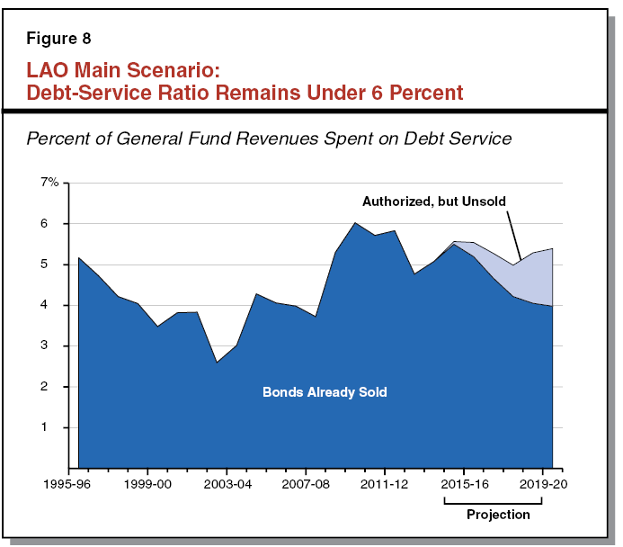
DSR Expected to Remain Under 6 Percent. Under our main scenario, the DSR remains under 6 percent over the next several years. We assume the state gradually sells bonds that previously have been approved by voters or the Legislature. These bonds include some of the remaining unsold infrastructure bonds that voters approved in 2006 and 2008, as well as a portion of the water bond approved in November 2014 (Proposition 1). We note that water bond sales are expected to occur over a number of years, so the water bond’s full annual debt–service costs will not occur until after the forecast period.

Chapter 4: Implementing Proposition 2

Passed on November 4, 2014, Proposition 2 changes the way the state pays down debt and saves money in reserves. The measure also creates a state reserve for Proposition 98 funding for schools and community colleges. In addition, in the year following a deposit to the new Proposition 98 reserve, Chapter 32, Statutes of 2014 (SB 858, Committee on Budget and Fiscal Review), establishes a maximum level of school district reserves. The Legislature could change this statutory provision in the future, unlike the rest of Proposition 2’s changes to the State Constitution. The effects of Proposition 2 may not be felt by schools and community colleges for at least a few years. The flowchart in Figure 1 shows how the new reserve and debt rules will affect state budget calculations.

Choices About Rules and Calculations

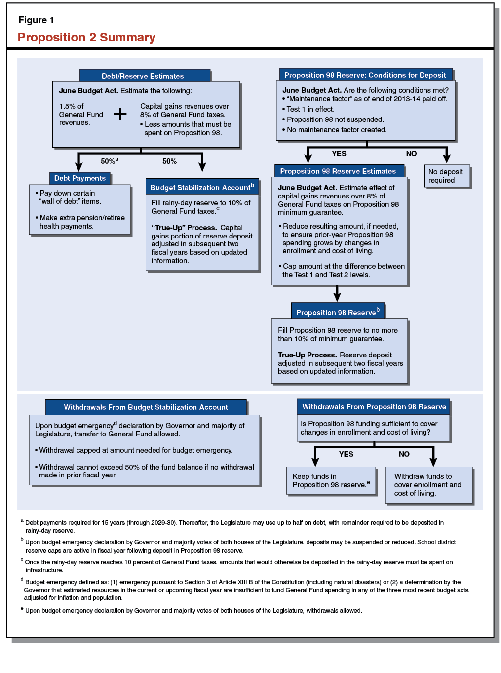
Highly Complex Interactions With Other Budget Formulas. Proposition 2 is highly complex and will influence key decisions concerning the state’s reserve and debt policies. Due to interactions with the Proposition 98 funding formula for schools and community colleges, Proposition 2 will sometimes produce results that are difficult to predict and counterintuitive. The state will have various choices to make when implementing Proposition 2. We list some of those key choices for policymakers in Figure 2 and discuss each below. (Figure 2 also lists the choices reflected in our fiscal outlook calculations when applicable.) Depending on the choices made by policymakers, reserve deposits and debt payments—and therefore the amount available for other state spending priorities—could vary by a billion dollars or more in a given fiscal year.

Pre–Proposition 2 BSA Deposits

Rules Concerning Control Over $1.6 Billion Deposited to BSA in 2014–15 Budget. Under Proposition 2, the state can access the Budget Stabilization Account (BSA) funds only when the Governor declares a budget emergency (the conditions for which are discussed later in this chapter). Proposition 2, however, does not explicitly apply these withdrawal rules to the $1.6 billion that was deposited in the BSA in the 2014–15 budget. There is, therefore, a strong argument that the Legislature has broad authority to use that $1.6 billion when and how it sees fit, similar to the flexibility provided under the State Constitution prior to Proposition 2’s passage. In general, the California Legislature has broad power unless the Constitution specifically constrains the legislative branch. Under this view, the $1.6 billion deposited to the BSA in 2014–15 could be appropriated without the Governor first declaring a Proposition 2 budget emergency. Alternatively, the Legislature and the Governor could choose to apply the new Proposition 2 rules to these funds, meaning the Governor would have to first declare a budget emergency before the Legislature could transfer the $1.6 billion back to the General Fund. The decision reached by the Governor and Legislature on how to treat this $1.6 billion could play a key role in determining the amount available for the Legislature in crafting the 2015–16 budget. Even if the state’s leaders agreed the $1.6 billion was not bound by Proposition 2’s rules on reserve withdrawals, they could leave all or some of this money untouched and, therefore, available to help the budget in a future economic downturn.

Capital Gains Calculations

Proposition 2 requires complex calculations be made concerning net capital gains taxes—a component of the personal income tax that is impossible to predict with any great certainty. Below, we describe decisions the state will face in administering various capital gains–related calculations in Proposition 2 and how these decisions could affect state reserve and debt payment requirements for 2015–16 and beyond.

Key Choice About Proposition 2 Calculation Affects Size of Reserve/Debt Payments. The text of Proposition 2 references constitutional school funding formulas, not statutory funding formulas. One of the statutory school funding formulas, however, can affect the Proposition 2 calculations—potentially having a significant impact on the size of the required BSA deposits and debt payments. Specifically, if the state were to apply the statutory formula for the Test 3 supplemental appropriation, the size of the BSA deposit/debt payments would be larger than if the state were not to use that formula in making its Proposition 2 calculations. Figure 3 provides an illustration of the effect of this choice. Under our main outlook scenario, applying the statutory Test 3 formula to the Proposition 2 calculations in 2015–16 results in a BSA deposit/debt payment requirement that is $1 billion higher in 2015–16 than the alternative approach, which excludes the formula from the Proposition 2 calculations. The Legislature will need to decide whether to apply this statutory supplemental formula in the state’s Proposition 2 calculations. It is important to note that the choice the Legislature makes in this matter will not affect school funding. It will only affect the amount available for deposits/debt payments versus the rest of the state budget.

Average vs. Marginal Tax Rates. California has a progressive rate structure with higher levels of income taxed at higher rates. For example, a single filer making over $500,000 a year pays a marginal tax rate of 12.3 percent on income above that level, but lesser rates on income below that amount. This results in an average tax rate on that individual’s total income that is less than the marginal rate. Calculating how much capital gains revenue is captured by Proposition 2 requires an assumption about whether average or marginal rates are used to estimate the amount of capital gains taxes. Although there is no right answer regarding this decision, estimates using average tax rates will be somewhat lower than those using marginal tax rates. (In this report, we assume an average tax rate in part because we understand this method was used by the administration in modeling Proposition 2 during legislative deliberations last spring.) If the state instead were to use marginal tax rates in its Proposition 2 calculations, the estimated amount of capital gains captured by Proposition 2 would be larger, meaning higher reserve and debt payment requirements of potentially hundreds of millions of dollars in years with high capital gains.

Attributing Capital Gains Taxes to Fiscal Years. Individuals generally pay taxes on a calendar–year basis while the state budgets its revenues and spending on a fiscal–year basis. For example, taxes paid in 2015 will generate revenues in two fiscal years—2014–15 and 2015–16. Accordingly, the state must make assumptions about how much tax revenue paid during a calendar year is applied to each fiscal year. These issues affect Proposition 2 because, for example, part of the capital gains earned by taxpayers in 2015 will go into the 2015–16 reserve and debt calculations. The administration’s current method assumes that 30 percent of the 2015 capital gains will be attributed to 2014–15, with the remaining 70 percent attributed to 2015–16. There is no single correct assumption in this regard, as tax dollars flowing into state coffers are not clearly “marked” as capital gains or non–capital gains dollars. There are probably several alternative measures that would split capital gains taxes between fiscal years reasonably for calculating Proposition 2’s reserve and debt requirements.

Estimating Methods Could Affect Debt Payments. We note that some prior administration revenue forecasts have assumed that future capital gains will match a long–term historical average of capital gains as a share of the state’s economy. This practice may have contributed to the administration’s more cautious revenue estimates in recent years. (That is, at times the administration’s capital gains projections seem to have relied as much or more on these historical averages as current or projected stock trends.) With regard to BSA deposits under Proposition 2, the state will subsequently true up capital gains revenues, providing an opportunity to deposit any capital gains taxes above initial projections in the state’s reserves. Debt payments, however, are not required to be adjusted when new capital gains estimates are available in subsequent years. A cautious capital gains estimating method therefore could result in less Proposition 2 debt payments over time because they may never be adjusted for subsequent increases in capital gains above initial projections.

Budget Emergency Fiscal Calculations

Choices Will Affect Availability of a Budget Emergency. Under Proposition 2, a budget emergency—when declared by the Governor—provides the Legislature with the flexibility to use BSA reserves or reduce BSA deposits. A budget emergency is available under Proposition 2’s fiscal calculations when estimated resources for the current or upcoming fiscal year are lower than the last three enacted budget spending totals, adjusted for population growth and inflation. As described in Chapter 1, under our estimates there would be no budget emergency available during the 2015–16 budget process based on the fiscal calculation described in Proposition 2. This, however, is subject to various choices that would affect whether a budget emergency can be declared by the Governor under Proposition 2’s fiscal calculations. We made the following choices in our calculations:

• Pre–Proposition 2 Deposits. Because there is a strong argument that the Legislature could appropriate funds from pre–Proposition 2 BSA deposits by a simple majority vote, we include as an estimated resource the $1.6 billion that was deposited to the BSA in the 2014–15 budget.
• Mandates Trigger. Because the $170 million mandates trigger was not included in official administration spending totals when the 2014–15 budget was enacted, we do not adjust the 2014–15 enacted budget total for that trigger.
• Proposition 2 Debt Payments. The state’s traditional estimate of resources available considers revenues but not expenditures. Some of the debts eligible for payment under Proposition 2—such as special fund loan repayments—are booked on the revenue side of the budget. Others—such as contributions to pension systems—appear on the spending side. As shown in Figure 1 of Chapter 3, we display “unallocated” Proposition 2 debt payments—those that are required by Proposition 2 but are not assumed elsewhere in our outlook—on the spending side of the budget. Placing these unallocated debt payments on the spending side is a choice we had to make in developing the calculations, since we cannot predict what type of debt payments these will be. Under the state’s traditional estimating practices, this choice means the unallocated debt payments do not affect estimated resources. Had we chose instead to book the unallocated debt payments on the revenue side of the budget, estimated resources would have been $695 million lower.

Near the end of Chapter 1, we displayed our budget emergency fiscal calculation, in which 2015–16 estimated resources were $2.1 billion above the adjusted 2014–15 spending level, thereby preventing a budget emergency under that calculation. If we had changed all three choices described above, this budget emergency calculation would be $2.5 billion “worse,” thereby allowing a budget emergency. This would allow the Governor to declare a budget emergency under Proposition 2’s fiscal calculations, and the Legislature to pass a 2015–16 budget that reduced or suspended deposits to the BSA.

Strategies for Paying Down Debt

Over the next 15 fiscal years, Proposition 2 could result in roughly $15 billion to $20 billion (in today’s dollars) being used to pay down state debts. These payments are mandatory for the next 15 years—that is, the Governor and the Legislature may not reduce these payments during a budget emergency. There are various strategies that the Legislature could employ for paying down state debts with the funds that are earmarked for that purpose by Proposition 2. In this section, we discuss how the Legislature can approach both its near–term and longer–term choices for using Proposition 2 debt payment funds.

Addressing Persistent State Debts

In our May 2014 report, Addressing California’s Key Liabilities, we discussed a wide variety of state debts. Figure 4 lists the specific categories of debts eligible for repayment using Proposition 2’s annual stream of earmarked funding over the next 15 years. (The May 2014 reports provides more information on these debts.)

Budgetary Liabilities. The state General Fund owes billions of dollars of budgetary debts to other state accounts (known as special funds), school districts, and other local governments. In general, these debts are owed because these entities helped the state balance its budget in prior years. The state has an obligation to repay each of the budgetary liabilities shown in Figure 4.

Retirement Liabilities Already Being Addressed. Many of the state’s retirement–related debts, including unfunded liabilities for state and the California State University (CSU) employee pensions, are being addressed with routine annual payments over time. We discussed how such debts are already being addressed in our May 2014 report. In June 2014, the Legislature approved a law that aims to fully fund the California State Teachers’ Retirement System (CalSTRS) unfunded pension liabilities over about 30 years. If Proposition 2 funds were used to pay down these debts more quickly than now planned, long–term taxpayer savings would result because a smaller portion of these liabilities would be passed to future taxpayers.

Retirement Liabilities Not Being Addressed. Various other state debts—including tens of billions of dollars of unfunded liabilities for health benefits of state government, CSU, and the University of California (UC) retirees—are not being addressed. The state, for example, does not set aside funds for the retiree health benefits accrued by its employees during their working lives. Instead, it pays for these retiree health benefits on a pay–as–you–go basis, which is a problematic and expensive way to address the issue. Taking action to pay retiree health liabilities with Proposition 2 funds could save taxpayers tens of billions of dollars over the long term. This action would result in a smaller portion of liabilities being passed to future taxpayers.

Suggested Approach

Plan Needed. We recommend that the Legislature develop a plan for use of the Proposition 2 debt payment funds. The plan could include near–term and longer–term elements, as summarized in Figure 5. As we discuss below, addressing the state’s retirement–related liabilities may involve significant logistical issues and trade–offs. Over the next year or two, the Legislature could work with the administration and state–level retirement systems on a plan to use Proposition 2 funds to address selected retirement liabilities in future years. In the meantime, beginning in 2015–16, the state could tackle a significant portion of the budgetary liabilities listed in Figure 4, as well as a difficult pension problem that has plagued the state for decades: the pension system for judges elected or appointed before November 1994 known as Judges’ Retirement System I (JRS I).

Judges’ Retirement System I. JRS I is administered by the California Public Employees’ Retirement System (CalPERS) separate from its other pension plans and has never been adequately funded. Currently, it is the state’s worst–funded pension system, with an unfunded liability of $3.3 billion and only 2 percent of assets needed to cover the system’s liabilities. The state essentially funds JRS I pension benefits on a pay–as–you–go basis. If the state were instead to fully fund JRS I over the next few years using Proposition 2 funds, the state’s existing pay–as–you–go requirements to the system would end. Annual General Fund savings of perhaps $200 million, declining slowly over time, would result after the JRS I unfunded liability is retired.

Suggested Near–Term Plan. We suggest that the Legislature pay down a significant portion of the eligible budgetary liabilities using Proposition 2 debt payment funds over the next few years. These funds would provide one–time resources for state special funds, school districts, and local governments. In addition, we think the Legislature should seriously consider addressing much or all of the JRS I unfunded liability over the next few years, which could provide General Fund budgetary savings in the fiscal years thereafter.

Developing a Long–Term Plan. It took the Legislature several years to develop the recent plan to address CalSTRS’ unfunded liabilities. Evaluating which of the state’s large retirement liabilities merit priority in a longer–term Proposition 2 plan deserves serious consideration. We suggest that the Legislature invite the administration, CalPERS, CalSTRS, UC, and other stakeholders to respond with proposals describing how Proposition 2 funds could help address one or more of the state’s large retirement–related debts over the next 15 years. Proposals should describe in detail the long–term public savings that would result from a commitment of Proposition 2 funds to a specific retirement liability. Within the next few years, the Legislature could take elements from one or more of these plans—or come up with its own plan—to address a portion of the state’s large, persistent retirement–related debts.

Opportunity to Address Retiree Health Liabilities. Not setting aside funds for retiree health benefits earned during employees’ working lives violates a fundamental tenet of public finance—that costs should be paid in the year when they are incurred. The state’s current pay–as–you–go retiree health funding system is much more costly than if the state funded those benefits as they were earned. Accordingly, reducing and eventually addressing unfunded retiree health liabilities of public entities could save taxpayers billions of dollars over the long term.

We have long recommended that the state and other public entities move toward funding retiree health liabilities properly. Proposition 2 provides the state with an intriguing opportunity to address a significant portion of these persistent debts over the next 15 years. Other long–term Proposition 2 plans—such as addressing CalPERS, CalSTRS, or UC pension liabilities—may have merit, but we urge the Legislature to give strong consideration to using the funds earmarked by Proposition 2 to pay state, CSU, and/or UC retiree health liabilities beginning a few years from now.

If it chose to use Proposition 2 debt payment funds to pay down retiree health liabilities, the state would have a number of significant logistical issues to consider over the next few years, including: (1) whether to increase fees of special funds that do not currently have the budgetary flexibility to fund their share of retiree health costs, (2) how to manage federal funding for the share of state employee costs funded by the U.S. government, (3) whether state employees should pay more to fund retiree health benefits, and (4) how a state retiree health trust fund would be administered. These issues would require detailed review by attorneys, tax experts, and others. As such, the Legislature may wish to act within the next few months to direct state entities to develop a plan for these matters so that Proposition 2 funds could be used for this purpose within the next few years.

Chapter 5: The State Budget After 2015–16

Multiyear Budget Outlooks Are Challenging. Estimating the future condition of California’s General Fund has long been a difficult task. Revenues—and some spending requirements, such as Proposition 98—are driven by volatile tax revenues and the ebbs and flows of the stock market and business income. Moreover, the highly complex interactions of Proposition 2 with the stock market, Proposition 98, and other elements of the budget are now increasing substantially the difficulty of producing multiyear budget outlooks. Finally, it is important for readers of this publication to recognize that we are not attempting to predict the actions of state policymakers and voters in the future. As we described earlier (see “Keys to Understanding This Report” in Chapter 1), we assume in our fiscal outlook publications that today’s laws and budget practices remain in place. The state’s leaders can use our estimates and other information to make decisions about changes in policies that may increase or decrease state spending or revenues. Because the state will make such policy changes over time, future estimates of revenue and spending will not be directly comparable to those in this report.

Outlook Scenarios Dependent on Assumptions Underlying Them. Considering all of the challenges described above, multiyear budget outlooks like the ones discussed in this publication depend on their underlying scenarios and assumptions. There are a variety of economic and revenue assumptions, for example, that one could adopt in considering the future of California’s budget. In this chapter, we describe how three different scenarios could affect the state budget outlook after 2015–16: (1) our main scenario (discussed through much of this publication) that assumes continuing, moderate economic growth through 2020, (2) an illustrative and purely hypothetical “slowdown scenario” that involves a significant stock market drop and much slower economic growth for a time beginning in 2016, and (3) another hypothetical scenario that considers a “temporary revenue surge” of the type California could experience in this fiscal year, if capital gains cause a temporary increase in state tax collections.

Main Scenario: Surpluses and Budget Reserves

Economic Assumption: Continuing, Moderate Growth. As discussed in Chapter 2, our main scenario—like those of many economic forecasters—assumes continuing, moderate growth over the next several years. We think our main scenario is a reasonable projection, based on what we observe at the present time, of near–term economic conditions relevant for the 2015–16 budget process. After 2015, however, the main scenario makes assumptions about future economic growth that may or may not come to pass. Even if economic growth continues in future years, that growth could be more or less than assumed in our main scenario in any fiscal year. This, in turn, has important implications for the state’s complex budgetary formulas—especially those of Proposition 98 and Proposition 2—the outcomes of which can change significantly with different economic inputs.

LAO Main Scenario Assumes Declining Capital Gains After 2014. California’s tax revenues have numerous volatile elements, but among the more significant sources of revenue volatility are the state’s tax levies on net capital gains through the personal income tax. Every budget outlook must make assumptions about Californians’ capital gains realizations, either explicitly or implicitly. In Figure 1, we display our assumptions, compared to those that the administration included in its May 2014 forecast. (The administration’s May 2014 assumptions were the basis of the state’s 2014–15 budget plan.) Figure 1 displays the total amount of net capital gains reported by California residents on their state tax returns through 2012 and our projections for tax years 2013 and beyond. (Final data for 2013 will not be available until sometime next year because some taxpayers just submitted their 2013 extension returns a few weeks ago and state tax officials require time to compile data from returns.) We assume in our main scenario that 2014 capital gains are spiking due to recent, large gains in the stock market. It is important to stress, however, that even such near–term capital gains projections are subject to significant error. Further, we assume that a slightly declining stock market will cause capital gains to decline noticeably in 2015 and that modest future growth in the stock market will cause a gradual decline in net capital gains reported on Californians’ tax forms through 2018, followed by basically no growth thereafter through 2020.

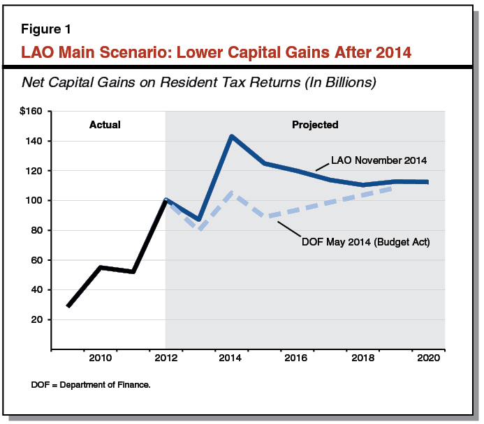
Under our main scenario’s Proposition 2 calculations, we assume that net capital gains taxes—determined with rough estimates of the average tax rates paid by taxpayers on the net gains shown in Figure 1—drop from $12.8 billion in 2014–15 to $11.4 billion in 2015–16, falling to $8.5 billion in 2019–20. By contrast, the administration’s May 2014 revenue forecasts assumed growth in capital gains after 2015, albeit from a lower base than the current high level of stock prices would seem to indicate. (In its June 2014 multiyear forecast of Proposition 2, for instance, the administration assumed that net capital gains taxes would be $9.4 billion in 2015–16 and grow to $10.5 billion in 2017–18.)

Surpluses and Reserves Accumulate in Main Scenario. Figure 2 shows our current outlook for the state’s General Fund under the main scenario, which assumes no additional budget policy commitments in the future. (Our main scenario, for example, reflects the spending listed in Figure 1 of Chapter 3.) For each fiscal year shown, the bar indicates the combined amount of the required deposit to the Proposition 2 Budget Stabilization Account (BSA), assuming no suspensions or reductions of those deposits, and budget surpluses (which would be available to build additional reserves or fund new budget commitments). In 2015–16, for example, our main scenario anticipates a nearly $2 billion BSA deposit and $641 million in available budget surpluses, which combine to equal the $2.6 billion bar for that fiscal year in Figure 2. Over the next three years, Proposition 2 BSA deposits generally decline due to our assumptions of lower capital gains after 2014, while the remaining surpluses increase. By 2019–20, the first year with no Proposition 30 revenues in our outlook, there is a $3 billion surplus and a $1 billion required BSA deposit. In this main scenario, the state’s BSA reserves would accumulate to about $8 billion by the end of 2019–20.

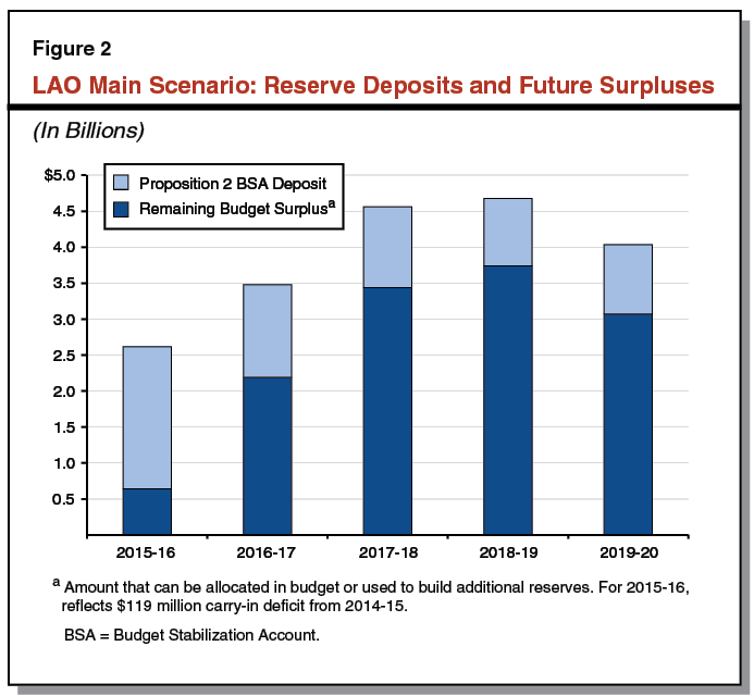
Surpluses Will Differ If New Budget Commitments Made. Relative to the budget picture reflected in Figure 2, one–time or ongoing changes to tax or spending policies will decrease or increase future surpluses and could affect required reserve deposits as well. Estimates in future editions of this publication will differ from those published here partly because of such future changes in policy. Changes in economic conditions also will affect future estimates.

Slowdown Scenario: Surpluses Evaporate

Big Stock Drop and Economic Slowdown: A Hypothetical Scenario. The U.S. economy is now into the sixth year of its current expansion—longer than the average expansion since World War II. Currently, we do not anticipate a major decline in the economy in 2014, 2015, or 2016, but it is very difficult to predict when the next economic downturn will occur or how severe it will be. Based on the historical length of economic expansions, it is likely that a significant economic slowdown or recession will occur prior to 2020. To illustrate the effect of a hypothetical slowdown on California’s budget condition, we developed a rough alternative slowdown scenario that assumes some weakness in the U.S. and California economies beginning in 2016. Most importantly for California’s tax base, the slowdown scenario assumes that stock prices drop about 20 percent during 2016. (Specifically, the S&P 500 stock index falls over 350 points in this scenario to levels it last recorded in June 2013.) The slowdown scenario assumes around 1 percent real gross domestic product (GDP) growth for the U.S. in 2016 and 2017 and 3.6 percent annual growth in California personal income during that period (much slower growth than under our main scenario). California unemployment rates begin to rise again by early 2017 as a part of the slowdown.

Under Hypothetical Slowdown, Surpluses Evaporate. Driven by large stock market–related losses, especially declines in capital gains taxes, surpluses in California’s General Fund evaporate in 2016–17 in the hypothetical slowdown scenario. The $4.2 billion in reserves that the state accumulates in 2015–16 in our main scenario could be enough to address a multibillion–dollar budget shortfall in 2016–17, but thereafter additional actions would be required to balance the General Fund budget. Figure 3 illustrates the shortfalls in this hypothetical exercise. As the figure shows, a $3.8 billion deficit in 2016–17 (consisting of shortfalls in both 2015–16 and 2016–17) could be covered by the $4.2 billion in reserves, leaving about $400 million still available for 2017–18.

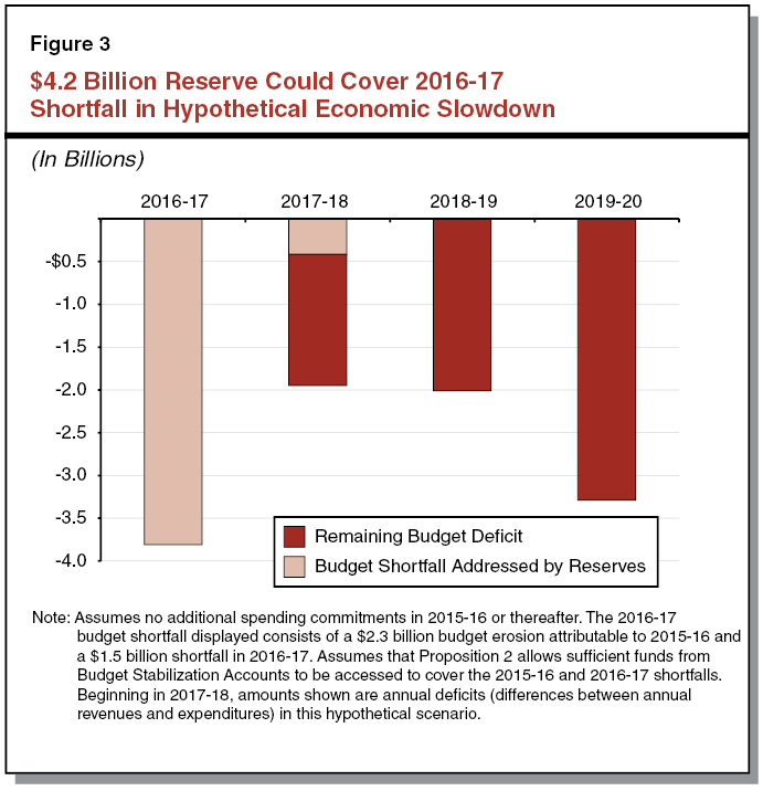
The remaining reserves likely would be exhausted in 2017–18, requiring state actions to address over $1 billion of a remaining budget shortfall. Thereafter, budget–balancing actions would be required to address annual deficits of $2 billion in 2018–19 and $3.3 billion in 2019–20. In the slowdown scenario, additional BSA deposits are assumed to be suspended beginning in 2016–17.

2015–16 Reserve Decisions Could Prove Crucial. The slowdown scenario is purely hypothetical. We are not predicting such a slowdown will occur within the next few years. Yet, economic and budget downturns rarely are predicted far in advance. Under the slowdown scenario, the budget reserves that we project could be accumulated by the state in 2015–16 might barely be enough to help the state through one year of a budget downturn. Thereafter, multibillion–dollar budget problems could return, requiring new decisions to return the state budget to balance. The shortfalls in the slowdown scenario are nowhere near the size of those that the state faced during the 2000s, but we stress that future economic slowdowns could be less severe or more severe than that in our hypothetical exercise. Our slowdown scenario, for instance, does not meet the classic definition of a recession, in that U.S. GDP does not fall in any two successive quarters. Rather, our slowdown scenario involves only one very small quarterly decline in GDP, accompanied by a number of quarters of very slow, but still slightly positive, growth. A harsher economic downturn—should it occur—could result in much more damage to the budget’s bottom line. The more reserves the state can accumulate in the near term, the better the state budget will be able to weather the next downturn.

Temporary Revenue Surge: Smaller Surpluses

Large One–Time Influx of Revenues: Another Hypothetical Scenario. Earlier in this publication, we described the significant possibility that 2014–15 personal income tax revenues will be higher than we indicate in our main scenario. To consider how such revenue increases could affect the General Fund’s future health, we assumed that everything in our main scenario was the same except for a temporary, capital gains–dominated “revenue surge” over the coming several months. Specifically, we assumed $1.5 billion more in revenues in 2014–15 and $500 million more in revenues in 2015–16, compared to our main scenario. We assumed that 75 percent of the additional revenues come from taxes on net capital gains.

Ongoing Higher School Costs Would Make It Harder to Balance Budget. Under the hypothetical revenue surge, the state’s Proposition 98 spending requirements would increase by $1.5 billion in 2014–15, taking up virtually all of the increased revenues. Perhaps more significantly, this $1.5 billion in higher school spending requirements would persist throughout our forecast period, generally reducing future surpluses after the temporary revenue gains disappear. For example, the $4.7 billion bar shown for 2018–19 in Figure 2 would be $1.4 billion smaller with this revenue surge due to a smaller budget surplus resulting from the higher Proposition 98 spending. Because of how it would ratchet up Proposition 98 spending, a temporary revenue surge in 2014–15 would mean lower surpluses and less money available for non–Proposition 98 spending commitments and non–BSA budget reserves throughout the forecast period. Such a temporary revenue spike would make the budget’s bottom line more vulnerable to future economic downturns. Under this hypothetical scenario, the amounts required to be deposited to the BSA under Proposition 2 would be slightly smaller in 2015–16 (about $200 million less than in the main scenario).

Complex Budget … Complex Outlook

Figure 4 lists some of the key numbers in the scenarios described in this chapter.

In conclusion, the state could see the condition of its General Fund—and its capacity either to build budget reserves or expand non–Proposition 98 budget commitments—worsen in the future if (1) revenues decline sharply or (2) revenues increase sharply, but temporarily, in 2014–15. The state’s future budget conditions will be marked at times by sharp declines in response to economic conditions, as well as some counterintuitive outcomes like those in the revenue surge scenario. Furthermore, the state’s budget can be affected by federal policy changes and cost trends in health care and other programs that we do not anticipate today. By accumulating budget reserves when state revenue growth is strong and carefully targeting any new budget commitments, the state’s policymakers can help keep the recently strengthened budget on a healthy track, despite these likely future challenges. Moreover, by using the Proposition 2 debt payment funds to tackle large, persistent debts over the next 15 years, the state’s policymakers can ensure more budget flexibility for the General Fund over the long term.