Introduction
For many California taxpayers, the property tax bill is one of the largest tax payments they make each year. For thousands of California local governments—K–12 schools, community colleges, cities, counties, and special districts—revenue from property tax bills represents the foundation of their budgets.
Although property taxes and charges play a major role in California finance, many elements of this financing system are complex and not well understood. The purpose of this report is to serve as an introductory reference to this key funding source. The report begins by explaining the most common taxes and charges on the property tax bill and how these levies are calculated. It then describes how the funds collected from property tax bills—$55 billion in 2010–11—are distributed among local governments. Last, because California’s property taxation system has evoked controversy over the years, the report provides a framework for evaluating it. Specifically, we examine California property taxes relative to the criteria commonly used by economists for reviewing tax systems, including revenue growth, stability, simplicity, neutrality, and equity. The report is followed with an appendix providing further detail about the allocation of property tax revenue.
What Is on the Property Tax Bill?
A California property tax bill includes a variety of different taxes and charges. As shown on the sample property tax bill in Figure 1, these levies commonly include:
- The 1 percent rate established by Proposition 13 (1978).
- Additional tax rates to pay for local voter–approved debt.
- Property assessments.
- Mello–Roos taxes.
- Parcel taxes.
The Constitution establishes a process for determining a property’s taxable value for purposes of calculating tax levies from the 1 percent rate and voter–approved debt. In our sample property tax bill, “Box A” identifies the taxable value of the property and “Box B” shows the property’s tax levies that are calculated based on this value. Levies based on value—such as the 1 percent rate and voter–approved debt rates—are known as “ad valorem” taxes.
Under the Constitution, other taxes and charges on the property tax bill (shown in “Box C”) may not be based on the property’s taxable value. Instead, they are based on other factors, such as the benefit the property owner receives from improvements.
As shown in “Box D,” the total amount due on most property tax bills is divided into two equal amounts. The first payment is due by December 10 and the second payment is due by April 10.
How Are Property Taxes and Charges Determined?
Ad valorem property taxes—the 1 percent rate and voter–approved debt rates—account for nearly 90 percent of the revenue collected from property tax bills in California. Given their importance, this section begins with an overview of ad valorem taxes and describes how county assessors determine property values. Later in the chapter, we discuss the taxes and charges that are determined based on factors other than property value.
Taxes Based on Property Value
The 1 Percent Rate. The largest component of most property owners’ annual property tax bill is the 1 percent rate—often called the 1 percent general tax levy or countywide rate. The Constitution limits this rate to 1 percent of assessed value. As shown on our sample property tax bill, the owner of a property assessed at $350,000 owes $3,500 under the 1 percent rate. The 1 percent rate is a general tax, meaning that local governments may use its revenue for any public purpose.
Voter–Approved Debt Rates. Most tax bills also include additional ad valorem property tax rates to pay for voter–approved debt. Revenue from these taxes is used primarily to repay general obligation bonds issued for local infrastructure projects, including the construction and rehabilitation of school facilities. (As described in the nearby box, some voter–approved rates are used to pay obligations approved by local voters before 1978.) Bond proceeds may not be used for general local government operating expenses, such as teacher salaries and administrative costs. Most local governments must obtain the approval of two–thirds of their local voters in order to issue general obligation bonds repaid with debt rates. General obligation bonds for school and community college facilities, however, may be approved by 55 percent of the school or community college district’s voters. Local voters do not approve a fixed tax rate for general obligation bond indebtedness. Instead, the rate adjusts annually so that it raises the amount of money needed to pay the bond costs.
Debt Approved by Voters Prior to 1978
The California Constitution allows local governments to levy voter–approved debt rates—ad valorem rates above the 1 percent rate—for two purposes. The first purpose is to pay for indebtedness approved by voters prior to 1978, as allowed under Proposition 13 (1978). Proposition 42 (1986) authorized a second purpose by allowing local governments to levy additional ad valorem rates to pay the annual cost of general obligation bonds approved by voters for local infrastructure projects. Because most debt approved before 1978 has been paid off, most voter–approved debt rates today are used to repay general obligation bonds issued after 1986 as authorized under Proposition 42.
Some local governments, however, continue to levy voter–approved debt rates for indebtedness approved by voters before 1978. While most bonds issued before the passage of Proposition 13 have been paid off, state courts have determined that other obligations approved by voters before 1978 also can be paid with an additional ad valorem rate. Two common pre–1978 obligations paid with voter–approved debt rates are local government employee retirement costs and payments to the State Water Project.
Voter–Approved Retirement Benefits. Voters in some counties and cities approved ballot measures or city charters prior to 1978 that established retirement benefits for local government employees. The California Supreme Court ruled that such pension obligations represent voter–approved indebtedness that could be paid with an additional ad valorem rate. Local governments may levy the rate to cover pension benefits for any employee, including those hired after 1978, but not to cover any enhancements to pension benefits enacted after 1978. Local governments may adjust the rate annually to cover employee retirement costs, but state law limits the rate to the level charged for such purposes in 1982–83 or 1983–84, whichever is higher. A recent review shows that at least 20 cities and 1 county levy voter–approved debt rates to pay some portion of their annual pension costs. The rates differ by locality. For example, the City of Fresno’s voter–approved debt rate for employee retirement costs is 0.03 percent of assessed value in 2012–13, while the City of San Fernando’s rate is 0.28 percent.
State Water Project Payments. Local water agencies can levy ad valorem rates above the 1 percent rate to pay their annual obligations for water deliveries from the State Water Project. State courts concluded that such costs were voter–approved debt because voters approved the construction, operation, and maintenance of the State Water Project in 1960. As a result, most water agencies that have contracts with the State Water Project levy a voter–approved debt rate.
Property tax bills often include more than one voter–approved debt rate. In our sample property tax bill, for example, the property owner is subject to four additional rates because local voters have approved bond funds for the city and water, school, and community college districts where the property is located. These rates tend to be a small percentage of assessed value. Statewide, the average property tax bill includes voter–approved debt rates that total about one–tenth of 1 percent of assessed value.
Calculating Property Value for Ad Valorem Taxes
One of the first items listed on a property tax bill is the assessed value of the land and improvements. Assessed value is the taxable value of the property, which includes the land and any improvements made to the land, such as buildings, landscaping, or other developments. The assessed value of land and improvements is important because the 1 percent rate and voter–approved debt rates are levied as a percentage of this value, meaning that properties with higher assessed values owe higher property taxes.
Under California’s tax system, the assessed value of most property is based on its purchase price. Below, we describe the process county assessors use to determine the value of local “real property” (land, buildings, and other permanent structures). This is followed by an explanation of how assessors determine the value of “personal property” (property not affixed to land or structures, such as computers, boats, airplanes, and business equipment) and “state assessed property” (certain business properties that cross county boundaries).
Local Real Property Is Assessed at Acquisition Value and Adjusted Upward Each Year. The process that county assessors use to determine the value of real property was established by Proposition 13. Under this system, when real property is purchased, the county assessor assigns it an assessed value that is equal to its purchase price, or “acquisition value.” Each year thereafter, the property’s assessed value increases by 2 percent or the rate of inflation, whichever is lower. This process continues until the property is sold, at which point the county assessor again assigns it an assessed value equal to its most recent purchase price. In other words, a property’s assessed value resets to market value (what a willing buyer would pay for it) when it is sold. (As shown in Figure 2, voters have approved various constitutional amendments that exclude certain property transfers from triggering this reassessment.)
Figure 2
Property Transfers That Do Not Trigger Reassessment
|
Proposition
|
Year
|
Description
|
|
3
|
1982
|
Allows property owners whose property has been taken by eminent domain proceedings to transfer their existing assessed value to a new property of similar size and function.
|
|
50
|
1986
|
Allows property owners whose property has been damaged or destroyed in a natural disaster to transfer their existing assessed value to a comparable replacement property within the same county.
|
|
58
|
1986
|
Excludes property transfers between spouses or between parents and children from triggering reassessment.
|
|
60
|
1986
|
Allows homeowners over the age of 55 to transfer their existing assessed value to a new home, of equal or lesser market value, within the same county.
|
|
90
|
1988
|
Extends Proposition 60 by allowing homeowners to transfer their existing assessed value to a new home, of equal or lesser market value, in a different participating county.
|
|
110
|
1990
|
Allows disabled homeowners to transfer their existing assessed value from an existing home to a newly purchased home of equal or lesser market value.
|
|
171
|
1993
|
Extends Proposition 50 by allowing property owners affected by a natural disaster to transfer their existing assessed value to a comparable replacement property in a different participating county.
|
|
193
|
1996
|
Excludes property transfers between grandparents and grandchildren (when the parents are deceased) from triggering reassessment.
|
|
1
|
1998
|
Allows property owners whose property is made unusable by an environmental problem to transfer their existing assessed value to a comparable replacement property.
|
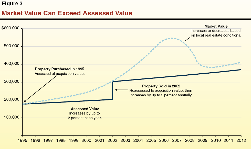
In most years, under this assessment practice, a property’s market value is greater than its assessed value. This occurs because assessed values increase by a maximum of 2 percent per year, whereas market values tend to increase more rapidly. Therefore, as long as a property does not change ownership, its assessed value increases predictably from one year to the next and is unaffected by higher annual increases in market value. For example, Figure 3 shows how a hypothetical property purchased in 1995 for $185,000 would be assessed in 2012. Although the market value of the property increased to $300,000 by 2002, the assessed value was $200,000 because assessed value grew by only up to 2 percent each year. Upon being sold in 2002, the property’s assessed value reset to a market value of $300,000. Because of the large annual increase in home values after 2002, however, the market value was soon much greater than the assessed value for the new owner as well.
Property Improvements Are Assessed Separately. When property owners undertake property improvements, such as additions, remodeling, or building expansions, the additions or upgrades are assessed at market value in that year and increase by up to 2 percent each year thereafter. The unimproved portion of the property continues to be assessed based on its original acquisition value. For example, if a homeowner purchased a home in 2002 and then added a garage in 2010, the home and garage would be assessed separately. The original property would be assessed at its 2002 acquisition value adjusted upward each year while the garage would be assessed at its 2010 market value adjusted upward. The property’s assessed value would be the combined value of the two portions. (As shown in Figure 4, voters have excluded certain property improvements from increasing the assessed value of a property.)
Figure 4
Property Improvements That Do Not Increase a Property’s Assessed Value
Constitutional Amendments Approved After June 1978
|
Proposition
|
Year
|
Type of Improvement
|
|
8
|
1978
|
Reconstruction following natural disaster
|
|
7
|
1980
|
Solar energy construction
|
|
31
|
1984
|
Fire–safety improvements
|
|
110
|
1990
|
Accessibility construction for disabled homeowners
|
|
177
|
1994
|
Accessibility construction for any property
|
|
1
|
1998
|
Reconstruction following environmental contamination
|
|
13
|
2010
|
Seismic safety improvements
|
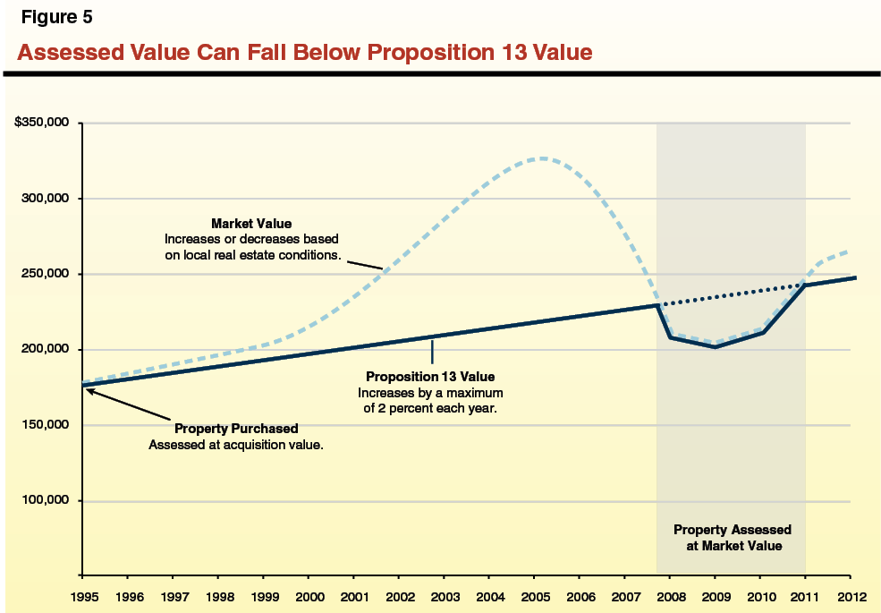
Assessed Value May Be Reduced When Market Values Fall Significantly. When real estate values decline or property damage occurs, a property’s market value may fall below its assessed value as set by Proposition 13. Absent any adjustment to this assessed value, the property would be taxed at a greater value than it is worth.
In these events, county assessors may automatically reduce the Proposition 13 assessed value of a property to its current market value. If they do not, however, a property owner may petition the assessor to have his or her assessed value reduced. These decline–in–value properties are often called “Prop 8 properties” after Proposition 8 (1978), which authorizes this assessment reduction to market value. Figure 5 illustrates the assessment of a hypothetical decline–in–value property over time. The market value of the property purchased in 1995 stays above its Proposition 13 assessed value through 2007. A significant decline, however, drops the property’s market value below its Proposition 13 assessed value. At this time, the property receives a decline–in–value assessment (equal to its market value) that is less than its Proposition 13 assessment. For three years, the property is assessed at market value, which may increase or decrease by any amount. By 2012, the property’s market value once again exceeds what its assessed value would have been absent Proposition 8 (acquisition price plus the 2 percent maximum annual increase). In subsequent years, the property’s assessed value is determined by its acquisition price adjusted upward each year.
Homeowners Are Eligible for a Property Tax Exemption. Homeowners may claim a $7,000 exemption from the assessed value of their primary residence each year. As shown in “Box A” of the sample property tax bill in Figure 1, this exemption lowers the assessed value of the homeowner’s land and improvements by $7,000, reducing taxes under the 1 percent rate by $70 and reducing taxes from voter–approved debt rates by a statewide average of $8.
Two Types of Property Are Assessed at Their Market Value. Two categories of property are assessed at their current market value, rather than their acquisition value: personal property and state– assessed property. (We provide more information about these properties in the nearby box.)Combined, these types of properties accounted for 6 percent of statewide–assessed value in 2011–12. Most personal property and state–assessed property is taxed at the 1 percent rate plus any additional rates for voter–approved debt.
Properties Assessed at Current Market Value
Personal Property. Personal property is property other than land, buildings, and other permanent structures, which are commonly referred to as “real property.” Most personal property is exempt from property taxation, including business inventories, materials used to manufacture products, household furniture and goods, personal items, and intangible property like gym memberships and life insurance policies. Some personal property, however, is subject to the property tax. These properties consist mainly of manufacturing equipment, business computers, planes, commercial boats, and office furniture. When determining the market value of personal property, county assessors take into account the loss in value due to the age and condition of personal property—a concept known as depreciation. Unlike property taxes on real property, which are due in two separate payments, taxes on personal property are due on July 3.
State–Assessed Property. The State Board of Equalization is responsible for assessing certain real properties that cross county boundaries, such as pipelines, railroad tracks and cars, and canals. State–assessed properties are assessed at market value and, with the exception of railroad cars, taxed at the 1 percent rate plus any additional rates for voter–approved debt. (As part of a federal court settlement decades ago, railroad cars are taxed at a rate that is somewhat lower than 1 percent. The railcar tax rate varies each year and currently is about 0.8 percent.)
Determining Other Taxes and Charges
All other taxes and charges on the property tax bill are calculated based on factors other than the property’s assessed value. For example, some levies are based on the cost of a service provided to the property. Others are based on the size of a parcel, its square footage, number of rooms, or other characteristics. Below, we discuss three of the most common categories of non–ad valorem levies: assessments, parcel taxes, and Mello–Roos taxes. In addition to these three categories, some local governments collect certain fees for service on property tax bills, such as charges to clear weeds on properties where the weeds present a fire safety hazard. These fees are diverse and relatively minor, and therefore are not examined in this report.
Assessments. Local governments levy assessments in order to fund improvements that benefit real property. For example, with the approval of affected property owners, a city or county may create a street lighting assessment district to fund the construction, operation, and maintenance of street lighting in an area. Under Proposition 218 (1996), improvements funded with assessments must provide a direct benefit to the property owner. An assessment typically cannot be levied for facilities or services that provide general public benefits, such as schools, libraries, and public safety, even though these programs may increase the value of property. Moreover, the amount each property owner pays must reflect the cost incurred by the local government to provide the improvement and the benefit the property receives from it. To impose a new assessment, a local government must secure the approval of a weighted majority of affected property owners, with each property owner’s vote weighted in proportion to the amount of the assessment he or she would pay.
Parcel Taxes. With the approval of two–thirds of voters, local governments may impose a tax on all parcels in their jurisdiction (or a subset of parcels in their jurisdiction). Local governments typically set parcel taxes at fixed amounts per parcel (or fixed amounts per room or per square foot of the parcel). Unlike assessments, parcel tax revenue may be used to fund a variety of local government services, even if the service does not benefit the property directly. For example, school districts may use parcel tax revenue to pay teacher salaries or administrative costs. The use of parcel tax revenue, however, is restricted to the public programs, services, or projects that voters approved when enacting the parcel tax.
Mello–Roos Taxes. Mello–Roos taxes are a flexible revenue source for local governments because they (1) may be used to fund infrastructure projects or certain services; (2) may be levied in proportion to the benefit a property receives, equally on all parcels, by square footage, or by other factors; and (3) are collected within a geographical area drawn by local officials.
Local governments often use Mello–Roos taxes to pay for the public services and facilities associated with residential and commercial development. This occurs because landowners may approve Mello–Roos taxes by a special two–thirds vote—each owner receiving one vote per acre owned—when fewer than 12 registered voters reside in the proposed district. In this way, a developer who owns a large tract of land could vote to designate it as a Mello–Roos district. After the land is developed and sold to residential and commercial property owners, the new owners pay the Mello–Roos tax that funds schools, libraries, police and fire stations, or other public facilities and services in the new community. Mello–Roos taxes are subject to two–thirds voter approval when there are 12 or more voters in the proposed district.
What Properties Are Taxed?
Property taxes and charges are imposed on many types of properties. These properties include common types such as owner–occupied homes and commercial office space, as well as less common types like timeshares and boating docks. In the section below, we describe the state’s property tax base—the types of real properties that are subject to the 1 percent rate and the share of total assessed value that each property type represents.
Due to data limitations, we do not summarize the tax bases of other taxes and charges. We note, however, that the property tax base for other taxes and charges is different from the tax base for the 1 percent rate. This is because the 1 percent rate applies uniformly to all taxable real property, whereas other taxes and charges are levied at various levels and on various types of property throughout the state (according to local voter or local government preferences). For example, if a suburban school district levies a parcel tax on each parcel in a residential area, the owners of single–family homes would pay a large share of the total parcel taxes. Accordingly, the school district’s parcel tax base would be more heavily residential than the statewide property tax base under the 1 percent rate (which applies to all taxable property).
What Properties Are Subject to the 1 Percent Rate?
Although most real property is taxable, the Constitution exempts certain types of real property from taxation. In general, these are government properties or properties that are used for non–commercial purposes, including hospitals, religious properties, charities, and nonprofit schools and colleges. California properties that are subject to the property tax, however, can be classified in three ways:
- Owner–occupied residential—properties that receive the state’s homeowner’s exemption, which homeowners may claim on their primary residence.
- Investment and vacation residential—residential properties other than those used as a primary residence, including multifamily apartments, rental condominiums, rental homes, vacant residential land, and vacation homes.
- Commercial—retail properties, industrial plants, farms, and other income–producing properties.
Distribution of the Tax Base for the 1 Percent Rate
Owner–Occupied Residential. In 2010–11, there were 5.5 million owner–occupied homes in California with a total assessed value of $1.6 trillion. As shown in Figure 6, owner–occupied residential properties accounted for the largest share—39 percent—of the state’s tax base for the 1 percent rate.
Investment and Vacation Residential. Although the majority of residential properties are owner occupied, many others are investment or vacation properties such as multifamily apartments, rental condominiums, rental homes, vacant residential land, and vacation homes. (We classify vacant residential land and vacation homes as investment properties because they are an investment asset for the owner, even if he or she does not receive current income from them.) In 2010–11, there were 4.2 million investment and vacation residential properties. The assessed value of these properties was about $1.4 trillion, which represents 34 percent of the state’s total assessed value.
Commercial. In 2010–11, there were approximately 1.3 million commercial properties in California. This amount includes about 600,000 retail, industrial, and office properties (such as stores, gas stations, manufacturing facilities, and office buildings). It also includes 500,000 agricultural properties and 200,000 other properties (gas, oil, and mineral properties and the private use of public land). While commercial properties represent a relatively small share of the state’s total properties, they tend to have higher assessed values than other properties. Therefore, as shown in Figure 6, these properties (which have a total assessed value of $1.2 trillion) account for 28 percent of the state’s property tax base.
Has the Distribution of the Property Tax Base Changed Over Time?
There is little statewide information regarding the composition of California’s property tax base over time. Based on the available information, however, it appears that homeowners may be paying a larger percentage of total property taxes today than they did decades ago. We note, for example, that the assessed value of owner–occupied homes has increased from a low of 32 percent of statewide assessed valuation in 1986–87 to a high of 39 percent in 2005–06. (The share was 36 percent in 2011–12.) It also appears likely that owners of commercial property are paying a smaller percentage of property taxes than they did decades ago. For example, Los Angeles County reports that the share of total assessed value represented by commercial property in the county declined from 40 percent in 1985 to 30 percent in 2012. In addition, the assessed value of commercial property in Santa Clara County has declined (as a share of the county total) from 29 percent to 24 percent since 1999–00.
What Factors May Have Contributed to Changes in the Property Tax Base?
Various economic changes that have taken place over time probably have contributed to changes to California’s property tax base. For example, investment in residential property has increased significantly since the mid–1970s. Newly built single–family homes have become larger and are more likely to have valuable amenities than homes built earlier. As a result, new homes are more expensive to build and assessed at higher amounts than older homes. Over the same period, commercial activity in California has shifted away from traditional manufacturing, which tends to rely heavily on real property. Newer businesses, on the other hand, are more likely to be technology and information services based. These businesses tend to own less real property than traditional manufacturing firms do. (Technology and information services firms, however, rely heavily on business personal property—for example, computing systems, design studios, and office equipment—that are taxed as personal property and not included in the distribution of the state’s real property tax base.)
It also is possible that Proposition 13’s acquisition value assessment system has played a role in the changes to California’s tax base. Specifically, under Proposition 13, properties that change ownership more frequently tend to be assessed more closely to market value than properties that turn over less frequently. (Because properties are assessed to market value when they change ownership, properties that have not changed ownership in many years tend to have larger gaps between their assessed values and market values.) It is possible that some categories of properties change ownership more frequently than others and this could influence the composition of the overall tax base. The limited available research suggests that investment and vacation residential properties change ownership more frequently than commercial or owner–occupied residential property, indicating that they may be assessed closer to market value than other types of property.
How Much Revenue Is Collected?
In 2010–11, California property tax bills totaled $55 billion. As shown in Figure 7, this amount included $43.2 billion under the 1 percent rate and $5.7 billion from voter–approved debt rates, making ad valorem property taxes one of California’s largest revenue sources.
Comparatively little is known about the remaining $6 billion of other taxes and charges on the property tax bill. From various reports summarizing local government finances, elections, and bond issuances, it appears that most of this $6 billion reflects property assessments, parcel taxes, and Mello–Roos taxes, though statewide data are not available on the exact amounts collected for each of these funding sources.
How Is the Revenue Distributed?
California property owners pay their property tax bills to their county tax collector (sometimes called the county treasurer–tax collector). The funds are then transferred to the county auditor for distribution. The county auditor distributes the funds collected from the 1 percent rate differently than the funds collected from the other taxes and charges on the bill. Specifically, the 1 percent rate is a shared revenue source for multiple local governments.
This section describes the distribution of revenue raised under the 1 percent rate and summarizes the limited available information regarding the distribution of voter–approved debt rates and non–ad valorem property taxes and charges.
Revenue From the 1 Percent Rate Is Shared by Many Local Governments
The 1 percent rate generates most of the revenue from the property tax bill—roughly $43 billion in 2010–11. On a typical property tax bill, however, the 1 percent rate is listed as the general tax levy or countywide rate with no indication as to which local governments receive the revenue or for what purpose the funds are used. In general, county auditors allocate revenue from the 1 percent rate to a variety of local governments within the county pursuant to a series of complex state statutes.
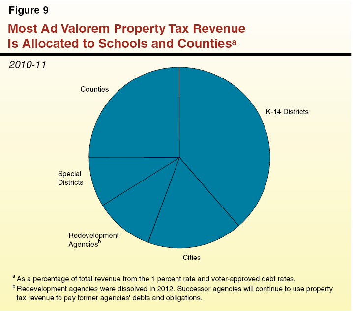
More Than 4,000 Local Governments Receive Revenue From the 1 Percent Rate. All property tax revenue remains within the county in which it is collected to be used exclusively by local governments. As shown in Figure 8, property tax revenue from the 1 percent rate is distributed to counties, cities, K–12 schools, community college districts, and special districts. Until recently, redevelopment agencies also received property tax revenue. As described in the nearby box, redevelopment agencies were dissolved in 2012, but a large amount of property tax revenue continues to be used to pay the former agencies’ debts and obligations.
Figure 8
How Many Local Governments Receive Revenue From the 1 Percent Rate?
|
Type of Local Government
|
Number
|
|
Counties
|
58
|
|
Cities
|
480
|
|
Schools and Community Colleges
|
|
|
K–12 school districts
|
966
|
|
County Offices of Education
|
56
|
|
Community college districts
|
72
|
|
Special Districts
|
|
|
Fire protection
|
348
|
|
County service area
|
316
|
|
Cemetery
|
241
|
|
Community services
|
201
|
|
Maintenance
|
136
|
|
Highway lighting
|
117
|
|
County water
|
100
|
|
Recreation and park
|
85
|
|
Hospital
|
64
|
|
Sanitary
|
60
|
|
Irrigation
|
46
|
|
Mosquito abatement
|
43
|
|
Public utility
|
43
|
|
Othera
|
400
|
|
Redevelopment Agenciesb
|
422
|
|
Total
|
4,254
|
Figure 9 shows the share of revenue received by each type of local government from the 1 percent rate and voter–approved debt rates. (As described later in the report, however, these shares vary significantly by locality.)
Redevelopment and Successor Agencies
More than 60 years ago, the Legislature established a process whereby a city or county could declare an area to be blighted and in need of redevelopment. After this declaration, most property tax revenue growth from the redevelopment “project area” was distributed to the redevelopment agency, instead of the other local governments serving the project area. As discussed in our report, The 2012–13 Budget: Unwinding Redevelopment, redevelopment agencies were dissolved in February 2012. Prior to their dissolution, however, redevelopment agencies received over $5 billion in property tax revenue annually. These monies were used to pay off tens of billions of dollars of outstanding bonds, contracts, and loans.
In most cases, the city or county that created the redevelopment agency is managing its dissolution as its successor agency. The successor agency manages redevelopment projects currently underway, pays existing debts and obligations, and disposes of redevelopment assets and properties. The successor agency is funded from the property tax revenue that previously would have been distributed to the redevelopment agency. As a result, even though redevelopment agencies have been dissolved, some property tax revenue continues to be used to pay redevelopment’s debts and obligations. Over time, most redevelopment obligations will be retired and the property tax revenue currently distributed to successor agencies will be distributed to K–14 districts, counties, cities, and special districts.
Property Taxes Also Affect the State Budget. Although the state does not receive any property tax revenue directly, the state has a substantial fiscal interest in the distribution of property tax revenue from the 1 percent rate because of the state’s education finance system. Each K–12 district receives “revenue limit” funding—the largest source of funding for districts—from the combination of local property tax revenue under the 1 percent rate and state resources. Thus, if a K–12 district’s local property tax revenue is not sufficient to meet its revenue limit, the state provides additional funds. Community colleges have a similar financing system, in which each district receives apportionment funding from local property tax revenue, student fees, and state resources. In 2010–11, the state contributed $22.5 billion to K–12 revenue limits and community college apportionments, while the remainder ($14.5 billion) came from local property tax revenue (and student fees).
State Laws Direct Allocation of Revenue From the 1 Percent Rate. The county auditor is responsible for allocating revenue generated from the 1 percent rate to local governments pursuant to state law. The allocation system is commonly referred to as “AB 8,” after the bill that first implemented the system—Chapter 282, Statutes of 1979 (AB 8, L. Greene). In general, AB 8 provides a share of the total property taxes collected within a community to each local government that provides services within that community. Each local government’s share is based on its proportionate countywide share of property taxes during the mid–1970s, a time when each local government determined its own property tax rate and property owners paid taxes based on the sum of these rates. (The average property tax rate totaled about 2.7 percent.) As a result, local governments that received a large share of property taxes in the 1970s typically receive a relatively large share of revenue from the 1 percent rate under AB 8. (More detail on the history of the state’s property tax allocation system—including AB 8—is provided in the appendix of this report.)
Revenue Allocated by Tax Rate Area (TRA). The county auditor allocates the revenue to local governments by TRA. A TRA is a small geographical area within the county that contains properties that are all served by a unique combination of local governments—the county, a city, and the same set of special districts and school districts. A single county may have thousands of TRAs. While there is considerable variation in the steps county auditors use to allocate revenue within each TRA, typically the county auditor annually determines how much revenue was collected in each TRA and first allocates to each local government in the TRA the same amount of revenue it received in the prior year. Each local government then receives a share of any growth (or loss) in revenue that occurred within the TRA that year. Each TRA has a set of growth factors that specify the proportion of revenue growth that goes to each local government. These factors—developed by county auditors pursuant to AB 8—are largely based on the share of revenue each local government received from the TRA during the late 1970s.
Figure 10 shows sample growth factors for TRAs in two California cities. As the figure indicates, 23 percent of any growth in revenue from the 1 percent rate in the sample TRA for Norwalk would be allocated to the county, 7 percent would go to the city, and the rest would be allocated to various educational entities and special districts. The percentage of property tax growth allocated to each type of local government can vary significantly by TRA. For example, Walnut Creek’s K–12 school district receives 33 percent of the growth in revenue within its TRA while Norwalk’s school district receives only 19 percent from its TRA. As noted above, this variation is based largely on historical factors specified in AB 8.
Figure 10
Allocation of Property Tax Growth in Sample Tax Rate Areas
|
Norwalk, Los Angeles Countya
|
Percent Share
|
|
Los Angeles County
|
23%
|
|
Educational Revenue Augmentation Fund
|
20
|
|
Norwalk–La Mirada Unified School District
|
19
|
|
Los Angeles County Fire Protection District
|
18
|
|
City of Norwalk
|
7
|
|
Norwalk Parks and Recreation District
|
3
|
|
Los Angeles County Library
|
2
|
|
La Mirada Parks and Recreation District
|
2
|
|
Cerritos Community College District
|
2
|
|
Los Angeles County Flood Control District
|
1
|
|
Los Angeles County Sanitation District
|
1
|
|
Greater Los Angeles County Vector Control
|
—b
|
|
Water Replenishment District of Southern California
|
—b
|
|
Little Lake Cemetery District
|
—b
|
|
Los Angeles County Department of Education
|
—b
|
|
|
100%
|
|
Walnut Creek, Contra Costa Countyc
|
Percent Share
|
|
Mount Diablo Unified School District
|
33%
|
|
Educational Revenue Augmentation Fund
|
17
|
|
Contra Costa County
|
13
|
|
Contra Costa County Fire
|
13
|
|
City of Walnut Creek
|
9
|
|
Contra Costa Community College District
|
5
|
|
East Bay Regional Park District
|
3
|
|
Contra Costa County Library
|
2
|
|
Central Contra Costa Sanitary District
|
2
|
|
Contra Costa County Office of Education
|
1
|
|
Contra Costa County Flood Control
|
1
|
|
Bay Area Rapid Transit
|
1
|
|
Contra Costa Water District
|
1
|
|
Contra Costa County Water Agency
|
—b
|
|
Contra Costa County Resource Conservation District
|
—b
|
|
Contra Costa County Mosquito Abatement District
|
—b
|
|
Contra Costa County Service Area R–8
|
—b
|
|
Bay Area Air Management District
|
—b
|
|
|
100%
|
Some Revenue Is Allocated to a Countywide Account—ERAF. Most of the revenue from the 1 percent rate collected within a TRA is allocated to the city, county, K–14 districts, and special districts that serve the properties in that TRA. State law, however, directs the county auditor to shift a portion of this revenue to a countywide account that is distributed to other local governments that do not necessarily serve the taxed properties. The state originally established this account—the Educational Revenue Augmentation Fund (ERAF)—to provide additional funds to K–14 districts that do not receive sufficient property tax revenue to meet their minimum funding level. State laws later expanded the use of ERAF to include reimbursing cities and counties for the loss of other local revenue sources (the vehicle license fee and sales tax) due to changes in state policy. For example, Figure 10 shows that 20 percent of any revenue growth within Norwalk’s TRA is deposited into ERAF. It is possible that some or all of this revenue could be allocated to a city or K–14 district in a different part of Los Angeles County.
Most Revenue From Voter–Approved Debt Distributed to Schools
Voter–approved debt rates are levied on property owners so that local governments can pay the debt service on voter–approved general obligation bonds (and pre–1978 voter–approved obligations). The state’s K–12 school districts receive the majority of the revenue from voter–approved debt rates ($3.1 billion of $5.2 billion in 2009–10). The amount received by cities ($520 million), special districts ($470 million), and counties ($320 million) is significantly less. The amount of taxes collected to pay voter–approved debt varies considerably across the state. For example, the average amount paid by an Alameda County property owner for voter–approved debt rates is about $2 for each $1,000 of assessed value, while the average amount paid in some counties is less than 10 cents per $1,000 of assessed value.
Limited Information About Distribution Of Other Property Taxes and Charges
Less information is available about the statewide distribution of the revenue from parcel taxes, Mello–Roos taxes, and assessments.
Parcel Taxes. Recent election reports and financial data suggest that parcel taxes represent a significant and growing source of revenue for some local governments. Specifically, between 2001 and 2012, local voters approved about 180 parcel tax measures to fund cities, counties, and special districts, and about 135 measures to fund K–12 districts. The most recent K–12 financial data (2009–10) indicate that schools received about $350 million from this source. We were not able to locate information on the statewide amount of parcel tax revenue collected by cities, counties, and special districts.
Mello–Roos Taxes. Mello–Roos districts are required to report on their bond issuance, which provides some information about the types of local governments that receive Mello–Roos tax revenue. It is likely that local governments issuing a large amount of Mello–Roos bonds also are collecting a large amount of Mello–Roos tax revenue. Between 2004 and 2011, cities issued about 50 percent of the bonds issued by Mello–Roos districts in California, followed by K–12 districts at about 30 percent. During the same time period, the issuance of Mello–Roos bonds was concentrated in specific regions, as more than 60 percent of the bonds were issued by local governments in four counties—Riverside, Orange, San Diego, and Placer.
Assessments. Most of the property improvements funded by assessments are provided by cities and special districts. In 2009–10, cities and special districts reported receiving $760 million and $650 million, respectively, in revenue from assessments. In contrast, counties reported $11 million in such revenues.
Why Do Local Government Property Tax Receipts Vary?
The share of revenue received by each type of local government from the 1 percent rate varies significantly by locality. County governments, for example, receive as little as 11 percent (Orange) and as much as 64 percent (Alpine) of the ad valorem property tax revenue collected within their county. As shown in Figure 11, revenue raised from the 1 percent rate also varies considerably by locality when measured by revenue per resident. Orange County receives about $175 per resident, while four counties receive more than $1,000 per resident. Although cities, on average, receive about $240 per resident in revenue from the 1 percent rate, some receive more than $500 per resident and many receive less than $150 per resident. School districts also receive widely different amounts of property taxes per enrolled student, with an average of just under $2,000. (As noted above, the state “tops off” school property tax revenue with state funds to bring most schools to similar revenue levels.) Finally, special districts also receive varying amounts of property tax revenue, though data limitations preclude us from summarizing this variation on a statewide basis.
Figure 11
Property Tax Receipts From the 1 Percent Rate for Selected Local Governments
2009–10
|
Cities
|
Property Taxes per Resident
|
Counties
|
Property Taxes per Resident
|
Schoolsa
|
Property Taxes per Student
|
|
Industry
|
$2,541
|
San Franciscob
|
$1,411
|
Mono
|
$10,683
|
|
Malibu
|
559
|
Sierra
|
1,126
|
San Mateo
|
5,432
|
|
Mountain View
|
344
|
Inyo
|
876
|
Marin
|
5,213
|
|
Los Angeles
|
332
|
Napa
|
522
|
San Francisco
|
4,020
|
|
Long Beach
|
268
|
El Dorado
|
464
|
Orange
|
3,315
|
|
Oakland
|
250
|
Los Angeles
|
359
|
San Diego
|
2,760
|
|
State Average
|
242
|
State Average
|
320
|
State Average
|
1,960
|
|
San Jose
|
200
|
Alameda
|
301
|
Yolo
|
1,765
|
|
Fresno
|
183
|
Sacramento
|
286
|
Sacramento
|
1,344
|
|
Anaheim
|
167
|
Contra Costa
|
271
|
San Joaquin
|
1,163
|
|
Santa Clarita
|
140
|
San Diego
|
261
|
Los Angeles
|
1,142
|
|
Chico
|
129
|
Riverside
|
200
|
Fresno
|
810
|
|
Modesto
|
119
|
Orange
|
174
|
Kings
|
379
|
Three factors account for most of this variation in local government property tax receipts. We discuss these factors below.
Variation in Property Values
California has a diverse array of communities with large variation in land and property values. Some communities are extensively developed and have many high–value homes and businesses, whereas others do not. Because property taxes are based on the assessed value of property, communities with greater levels of real estate development tend to receive more property tax revenue than communities with fewer developments. For example, high–density cities generally receive more property tax revenue than rural areas due to the greater level of development. Coastal and resort areas also typically receive more property taxes due to the high property values. Certain high–value properties—such as a power plant or oil refinery—also increase property tax revenue. Alternatively, localities with large amounts of land owned by the federal government, universities, or other organizations that are not required to pay property taxes may receive less revenue.
Prior Use of Redevelopment
Prior decisions by cities and counties to use redevelopment also influences the amount of property tax revenue local governments receive. Prior to the dissolution of redevelopment agencies in 2012, most of the growth in property taxes from redevelopment project areas went to the redevelopment agency, rather than other local governments. A large share of property tax revenue now goes to successor agencies to pay the former redevelopment agencies’ debts and obligations. The use of redevelopment varied extensively throughout the state. In those communities with many redevelopment project areas, the share of property tax revenue going to other local governments is less than it would be otherwise. In places with large redevelopment project areas—such as San Bernardino and Riverside counties—more than 20 percent of the county’s property tax revenue may go to pay the former redevelopment agencies’ debts and obligations.
State Allocation Laws Reflecting 1970s Taxation Levels
Finally, the amount of property taxes allocated to local governments depends on state property tax allocation laws, principally AB 8. As discussed earlier in this report (and in more detail in the appendix), the AB 8 system was designed, in part, to allocate property tax revenue in proportion to the share of property taxes received by a local government in the mid–1970s. Under this system, local governments that received a large share of property taxes in the 1970s typically continue to receive a relatively large share of property taxes today. Although there have been changes to the original property tax allocation system contained in AB 8, the allocation system continues to be substantially based on the variation in property tax receipts in effect in the 1970s.
This variation largely reflects service levels provided by local governments in the 1970s. Local governments providing many services generally collected more property taxes in the 1970s to pay for those services. As a result, those local governments received a larger share of property taxes under AB 8. For example, cities and counties that provided many government services, including fire protection, park and recreation programs, and water services, typically receive more property tax revenue than governments that relied on special districts to provide some or all of these services.
Are There Concerns About How Property Taxes Are Distributed?
While no system for sharing revenues among governmental entities is perfect, the state’s system for allocating property tax revenue from the 1 percent rate raises significant concerns about local control, responsiveness to modern needs, and transparency and accountability to taxpayers. We discuss these concerns separately below and then address the question: Could the state change the allocation system?
Lack of Local Control
Unlike local communities in other states, California residents and local officials have virtually no control over the distribution of property tax revenue to local governments. Instead, all major decisions regarding property tax allocation are controlled by the state. Accordingly, if residents desire an enhanced level of a particular service, there is no local forum or mechanism to allow property taxes to be reallocated among local governments to finance this improvement. For example, Orange County currently receives a very low share of property taxes collected within its borders—about 11 percent. If Orange County residents and businesses wished to expand county services, they have no way to redirect the property taxes currently allocated to other local governments. Their only option would be to request the Legislature to enact a new law—approved by two–thirds of the members of both houses—requiring the change in the property tax distribution. In other words, local officials have no power to raise or lower their property tax share on an annual basis to reflect the changing needs of their communities. As a result, if residents wish to increase overall county services, they would need to finance this improvement by raising funds through a different mechanism such as an assessment or special tax.
Limited Transparency and Accountability
The state’s current allocation system also makes it difficult for taxpayers to see which entities receive their tax dollars. Property tax bills note only that a bulk of the payment goes to the 1 percent general levy. Even if taxpayers do further research and locate the AB 8 local government sharing factors for their TRA, it is difficult to follow the actual allocation of revenue because the fund shifts related to ERAF and redevelopment complicate this system.
In addition to making it difficult for taxpayers to determine how their tax dollars are distributed, the AB 8 system reduces government accountability. The link between the level of government controlling the allocation of the tax (the state) and the government that spends the tax revenue (cities, counties, special districts, and K–14 districts) is severed. For example, if a taxpayer believes the level of services provided by an independent park district is inadequate, it is difficult to hold the district entirely accountable because the state is responsible for determining the share of property taxes allocated to the district.
Limited Responsiveness to Modern Needs and Preferences
An effective tax allocation system ensures that local tax revenue is allocated in a way that reflects modern needs and preferences. In many ways, California’s property tax allocation system—which remains largely based on allocation preferences from the 1970s—does not meet this criterion. California’s population and the governance structure of many local communities have changed significantly since the AB 8 system was enacted. For example, certain areas with relatively sparse populations in the 1970s have experienced substantial growth and many local government responsibilities have changed. One water district in San Mateo County—Los Trancos Water District—illustrates the extent to which the state’s property tax allocation system continues to reflect service levels from the 1970s. Specifically, this water district sold its entire water distribution system to a private company in 2005, but continues to receive property tax revenue for a service it no longer provides.
Changing the Allocation System Is Difficult
Over the years, the Legislature, local governments, the business community, and the public have recognized the limitations inherent in the state’s property tax allocation system. Despite the large degree of consensus on the problems, major proposals to reform the allocation system have not been enacted due to their complexity and the difficult trade–offs involved. Because California has thousands of local governments—many with overlapping jurisdictions—reorienting the property tax allocation system would be extraordinarily complex. Updating the AB 8 property tax sharing methodology would require the Legislature to determine the needs and preferences of each California community and local government. This would be a difficult—if not impossible—task to undertake in a centralized manner. Alternatively, the state could allow the distribution of the property tax to be carried out locally, but there is no consensus about what process local governments would use to allocate property taxes among themselves. Whether done centrally or locally, any reallocation is difficult because providing additional property tax receipts to one local government would require redirecting it from another local government or amending the Constitution. In addition, any significant change to the allocation of property tax revenue would require approval by two–thirds of the Legislature due to provisions in the Constitution added by Proposition 1A (2004). (These issues are discussed further in the appendix.)
What Are the Strengths and Limitations of California’s Property Tax System?
For many years, California’s overall property tax system—the types of taxes paid by property owners and the determination of property owner tax liabilities—has evoked controversy. Some people question whether the distribution of the tax burden between residential and commercial properties is appropriate and whether the amount of taxes someone pays should depend, in part, on how long he or she has owned the property. Other people praise the financial certainty that the tax system gives property owners. From one year to the next, property owners know that their tax liabilities under the 1 percent rate will increase only modestly. In this section, we do not attempt to resolve this long–standing debate. Instead, we review property taxes by looking at how they measure according to five common tax policy criteria—growth, stability, simplicity, neutrality, and equity. Using this framework, we highlight particular aspects of the state’s property tax system, both its strengths and limitations, for policymakers and other interested parties.
Economists use the five common tax policy criteria summarized in Figure 12 to objectively compare particular taxes. These criteria relate to how taxes affect people’s decisions, how they treat different taxpayers, and how the revenue raised from taxes performs over time. In practice, all taxes involve trade–offs. Sometimes the trade–offs are between two tax policy criteria. For example, revenue sources that grow quickly may be less stable from one year to the next than other revenue sources. Other times, the trade–offs are between tax policy criteria and other governmental policy objectives that may not be directly related to one of the five tax criteria. For example, one such trade–off might be that ensuring that a property owner’s taxes do not increase dramatically from one year to the next (a reasonable governmental policy objective) can result in a tax system in which the owners of similar properties are taxed much differently (contrary to the equity criteria of tax policy).
Figure 12
Common Economic Criteria for Evaluating Tax Systems
- Growth—Does revenue raised by the tax grow along with the economy or the program responsibilities it is expected to fund?
|
- Stability—Is the revenue raised by the tax relatively stable over time?
|
- Simplicity—Is the tax simple and inexpensive for taxpayers to pay and for government to collect?
|
- Neutrality—Does the tax have little or no impact on people’s decisions about how much to buy, sell, and invest?
|
- Equity—Do taxpayers with similar incomes pay similar amounts and do tax liabilities rise with income?
|
What Factors Affect Property Tax Growth Each Year?
Most of the annual change in property tax revenues is the result of large changes in assessed value that affect a small number of properties, including:
- Recently Sold Properties. When a property sells, its assessed value resets to the purchase price. This represents additional value that is added to the tax base because the sale price of the property is often much higher than its previous assessed value.
- Newly Built Property and Property Improvements. New value is added to the county’s tax base when new construction takes place or improvements are made—mainly additions, remodels, and facility expansions—because structures are assessed at market value the year that they are built.
- Proposition 8 (1978) Decline–in–Value Properties. These properties contribute significantly to growth or decline in a county’s tax base because their assessed values may increase or decrease dramatically in any year. A particularly large impact on assessed valuation tends to occur in years when a large number of these properties transfer from Proposition 13 assessment to reduced assessment.
As shown by the dark bars in the figure below, recently sold, newly built, and decline–in–value properties typically account for more than two–thirds of total changes in countywide assessed value in Santa Clara County. Other properties, although they represent most of the properties in the county’s tax base, contribute less because the growth of these properties’ assessed values is limited to 2 percent per year.
What Factors Affect Property Tax Stability?
Acquisition Value Assessment System Contributes to Revenue Stability.The main reason California’s property tax revenue is stable is that the assessed value of most properties increases each year by a maximum of 2 percent. In any given year, only a small fraction of properties are sold and reset to market value. This means that real estate conditions affect a relatively small portion of the tax base each year, insulating property tax revenue from year–to–year real estate fluctuations.
Proposition 8 (1978) Decline–in–Value Properties Reduce Revenue Stability. As noted earlier in the report, county assessors may reduce a property’s assessed value in the event that its market value falls below its assessed value. Each year thereafter, the property is assessed at market value until it rises above what its assessed value would have been had it remained at its acquisition value adjusted upward each year at a maximum of 2 percent. During 2010–11, more than one in four properties in California was temporarily assessed to market value. Because these properties are assessed each year at market value, they link the property tax base more closely to the local real estate market than other properties, thereby reducing the property tax’s stability somewhat.
Revenue Growth
From government’s perspective, revenue sources that grow along with the economy are preferable because they can provide resources sufficient to maintain current services. This can help governments avoid increasing existing taxes or taxing additional activities in order to meet current service demands.
The Property Tax Has Grown Faster Than the Economy. Personal income in California—an approximate measure of the size of the state’s economy—has grown at an average annual rate of 6.3 percent since 1979. Over the same period, revenue from the 1 percent property tax rate has grown at an average annual rate of 7.3 percent. As we describe in the nearby box, much of the growth in property tax revenue depends on new construction and property sales.
The Growth of Parcel and Mello–Roos Tax Revenues Depends on the Structure of the Tax. The terms of parcel taxes and Mello–Roos taxes vary by locality. Some local governments have taxes with escalation clauses or other provisions that modify the amount of the tax as local government costs change. Other parcel taxes and Mello–Roos taxes are set at fixed amounts per parcel. Depending on their structure, these taxes may or may not provide local governments with a growing source of revenue.
Revenue Stability
Revenue sources that remain relatively stable from one year to the next help governments manage economic downturns, which tend to reduce revenue and at the same time increase demand for certain public services. Stable revenue sources also may help governments plan more effectively for future needs, including long–term investments in transportation, education, and public safety.
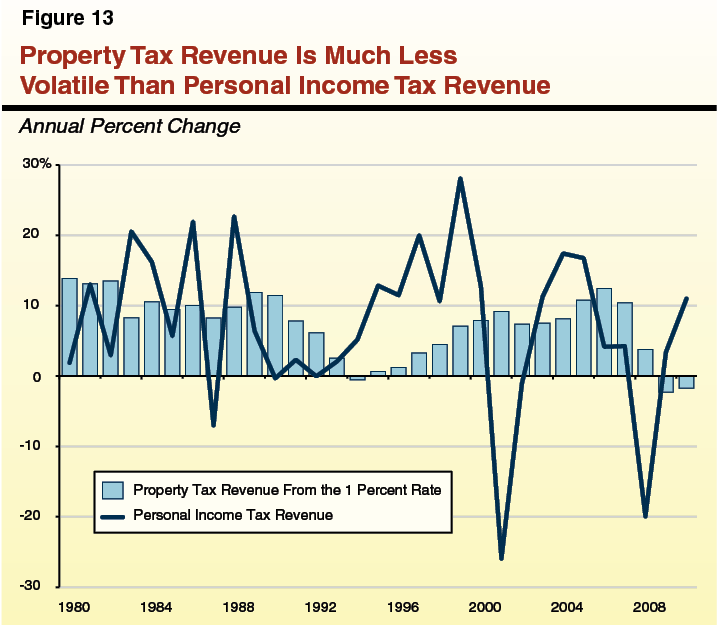
The Property Tax Is a Stable Revenue Source. Despite being linked to the volatile real estate market, the property tax is California’s most stable major revenue source. Since 1979, as shown in Figure 13, personal income tax revenue has been three times more volatile, on average, than property tax revenue from the 1 percent rate. During the same period, statewide property tax revenue has declined in only three years, 1994–95, 2009–10, and 2010–11.
The Property Tax Was More Stable Than Other Revenue Sources During the Recent Recession. As shown in Figure 14, revenue from the 1 percent property tax rate fared comparatively well during the most recent recession. (In the nearby box, we discuss why the property tax is stable.) Changes in property tax revenue tend to lag economic trends by one or more years because of the state’s acquisition value assessment system and the lengthy period between when most properties are assessed (January) and when property tax payments are due (December of that year and April of the next).
Parcel Taxes and Mello–Roos Taxes Also Are Stable. Because most parcel and Mello–Roos taxes are set at fixed amounts per parcel, there is minimal year–to–year fluctuation in the revenues that they raise.
Assessed Valuation in Some Counties, However, Has Declined Significantly. Though statewide property tax revenue has remained comparatively stable throughout the recent recession, some areas of the state have experienced considerable declines in their property tax base. These counties tend to have a large proportion of their properties under Proposition 8 decline–in–value assessments and have high foreclosure rates. For example, Riverside County had the second highest number of foreclosures (17,000) among counties and more than 400,000 decline–in–value properties in 2011. Partly as a result of these trends, total assessed value in Riverside County declined by 15 percent between 2008 and 2011.
Simplicity
A well–designed tax system should be simple for taxpayers to understand and easy and inexpensive for governments to administer. Complex tax systems can be expensive for governments to administer effectively and may be confusing, time–consuming, and costly for taxpayers.
Most of the costs associated with administering the state’s property tax system (ad valorem property taxes, parcel taxes, and Mello–Roos taxes) reflect the activities by county assessors, tax collectors, and auditors. While comprehensive data on these costs are not available, total property tax administration costs likely are between 1.5 percent and 2 percent of collections, a somewhat higher level than that of state tax agencies that perform similar functions. A significant component of the property tax’s administrative cost is from counties’ responsibility to allocate property taxes to local governments pursuant to increasingly complex state laws. County costs related solely to determining property values, the other main component of administration, were slightly less than 1 percent of total revenues collected in 2010–11—a percentage similar to that of state tax agencies.
From the taxpayers’ perspective, the property tax is generally a simple tax with which to comply. Tax payments are due in equal installments twice per year. And, in most years, the assessed value of real property grows automatically by a maximum of 2 percent. Reassessments based on market value (which taxpayers are more likely to appeal) occur infrequently for most property owners.
The property tax assessed on personal property is typically more administratively cumbersome for owners and assessors. This is because personal property is assessed annually at market value using complex depreciation schedules. These assessments, therefore, are more likely to be appealed, a process that can take more than a year to resolve.
Neutrality
Nearly all taxes alter taxpayer behavior to some degree. Economists agree, however, that in most cases the ideal tax system is one that alters decisions—about what goods to buy, what products to make, and where to work or live—as little as possible. Economists prefer these “economically neutral” taxes because they assume that people and businesses are in the best position to make consumption, savings, and investment decisions that meet their economic and personal needs. Tax policies that influence what people buy and what businesses produce tend to distance people and businesses from their preferred choices, leaving them less well off than they would be if the tax system were economically neutral. Policymakers design some taxes, on the other hand, to influence taxpayer behavior in a way that promotes or discourages particular activities. In general, these should be well targeted and have strong justifications so that they achieve their policy goals with as little interference as possible in other personal decision making. Below, we describe how ad valorem property taxes may influence taxpayer behavior and then discuss the possible effects of parcel and Mello–Roos taxes.
Some Homeowners and Businesses May Move Less Frequently. California’s ad valorem property taxes may affect an individual’s decision to move because longer ownership results in a lower effective property tax rate. (An effective property tax rate differs from the 1 percent basic rate in that it is the amount of property taxes paid divided by the current market value of the property.) As shown in Figure 15, effective tax rates can vary considerably. New Owner A, for example, has an effective tax rate of 1 percent because the assessed value of his or her property is the same as its market value. Owners B and C, who have owned their properties longer than Owner A, have assessed values below their market values because their market values increased by more than 2 percent each year (and therefore faster than assessed values). As a result, most owners who have owned a property for many years pay an effective tax rate well below 1 percent. For those choosing to move, however, their effective tax rate is reset to 1 percent, producing a moving penalty that may influence some property owners’ relocation decisions. For example, established firms that benefit from their comparatively low effective property tax rates could be dissuaded from relocating—decisions that, absent the moving penalty, could benefit the companies financially. (As we discuss below, differing effective tax rates also affect the equity of the property tax.)
Figure 15
Hypothetical Effective Property Tax Rates for Three Property Owners
|
|
Year Purchased
|
Market Value
|
Assessed Value
|
Property Tax Rate
|
Property Tax Paid
|
Effective Tax Rate
|
|
Owner A
|
2012
|
$300,000
|
$300,000
|
1%
|
$3,000
|
1.0%
|
|
Owner B
|
2002
|
300,000
|
180,000
|
1
|
1,800
|
0.6
|
|
Owner C
|
1986
|
300,000
|
110,000
|
1
|
1,100
|
0.4
|
Homeowners and Businesses May Invest Less in Property Improvements. When a property undergoes improvements, the newly constructed portion of the property is assessed at its full market value. The existing property, on the other hand, is typically assessed below its current market value, meaning that improvements are taxed at a higher effective rate than existing property. Because improvements are subject to higher effective tax rates, the return on investment that businesses receive from new improvements is lower and the taxes that homeowners pay on them are higher than they would be if all property—new and existing—were taxed uniformly. This may lead some businesses and homeowners to invest less than they otherwise would in new property improvements.
Homeowners May Change Behavior in Response to Assessment Exclusions. Voters have approved ballot propositions that exclude some types of property transfers from triggering reassessment to market value. (These exclusions are summarized earlier in this report in Figure 2.) For example, residential property transfers between certain family members do not trigger reassessment. These exclusions could alter decisions homeowners make about their property. For example, a homeowner might transfer property to his or her child (thereby passing on his or her low effective property tax rate) when, absent the exclusion, the owner might have sold the property to a nonrelative. In turn, that child could find it more economical to rent the property (and benefit from the low effective property tax rate) than to sell (and forego the benefit of his or her low effective rate).
Equity
Equity relates to how taxes affect taxpayers with different levels of income or wealth. Economists use two different standards of equity—vertical and horizontal—to evaluate taxes. Vertical equity occurs when wealthier taxpayers pay a greater amount in taxes than less wealthy taxpayers. Horizontal equity, on the other hand, occurs when similar taxpayers—those with similar incomes or wealth—pay the same amount in taxes. Under an equitable property tax system (1) owners of highly valuable property pay more in taxes than owners of less valuable property and (2) the owners of two similar properties pay a similar amount in property taxes. Put differently, an equitable system would tax property owners at the same effective rate. As we discussed in the previous section, however, property owners often are subject to different effective tax rates. Therefore, California’s ad valorem property taxes, parcel taxes, and Mello–Roos taxes often do not meet these standards of equity.
Equity Reduced by Acquisition Value Assessment and 2 Percent Assessed Value Cap. California’s property tax system does not consistently meet the standards of horizontal or vertical equity. As discussed earlier in this report, two owners with identical properties may pay different amounts of property taxes if one owner bought the property a decade before the other. In a tax system with horizontal equity, both owners would pay similar amounts. In relation to vertical equity, the tax system’s reliance on acquisition value and the 2 percent cap on assessed valuation growth can result in owners of valuable property paying less than owners of (recently acquired) less valuable property. In a tax system with vertical equity, owners of valuable property would pay more in taxes because owners of valuable property generally are wealthier than owners of less valuable property.
Homeowners Who Are Mobile Pay Higher Effective Tax Rates. Homeowners who move often—military families, younger homeowners, or those with jobs that require them to relocate frequently—tend to have higher effective ad valorem tax rates than homeowners who move less frequently because newly purchased properties are assessed at market value. Relocation decisions may result from circumstances that households may not have foreseen, such as employment changes, divorce, or other changes in family composition. Under horizontal equity, in contrast, taxpayers pay similar taxes unless their household income, wealth, or consumption patterns differ.
Fixed–Rate Taxes Do Not Meet Vertical Equity Standard. Parcel taxes and Mello–Roos taxes typically meet the criteria of horizontal equity but not vertical equity because property owners typically are charged the same amounts—regardless of their wealth or their properties’ value.
Summary
Our comparison of California’s property tax system with common tax policy criteria found mixed results. The ad valorem taxes generally meet the goals of administrative simplicity and providing governments with a growing source of stable revenue, but often do not meet the goals of neutrality and equity. Specifically, California’s ad valorem tax system (1) may influence decisions property owners make about relocations and expansions and (2) treat similar taxpayers differently and wealthier taxpayers the same as less wealthy taxpayers.
California’s other property taxes (parcel taxes and Mello–Roos taxes) generally perform well relative to the goals of stability, administrative simplicity, and horizontal equity, but may perform less well in regard to the other objectives.
Appendix 1: The History of California’s Property Tax Allocation System
California’s system for allocating property tax revenue from the 1 percent rate among local governments is complex and has changed over time. The most significant change was voter approval of Proposition 13 in 1978, which shifted the control over the allocation of property taxes from local communities to the state. Since that time the state has made several major changes that affect the amount of property tax revenue from the 1 percent rate distributed to counties, cities, K–14 districts, and special districts. Some of these changes have benefited the state fiscally (by indirectly reducing state costs for education). Others have benefited local governments or taxpayers. This appendix describes the evolution of the state’s property tax allocation system. The key events are highlighted in Figure A–1, and described in more detail below.
Figure A–1
History of California’s Property Tax Allocation
|
1972
|
SB 90—Establishes school “revenue limit” funding system, giving the state a significant fiscal interest in the allocation of local property tax revenue.
|
|
1978
|
Proposition 13—Voters cap the basic property tax rate at 1 percent and give the state new responsibilities for allocating property tax revenue.
|
|
|
SB 154—State’s first law allocating property tax revenue. Amounts based on share of property tax received prior to Proposition 13, with state providing grants for some of local revenue loss.
|
|
1979
|
AB 8—State changes property tax allocations in SB 154, establishes system for allocating future growth in property tax revenue, and absorbs costs of some local programs.
|
|
|
|
1992
|
First ERAF Shift—State permanently shifts some property tax revenue from counties, cities, and special districts into a fund for K–14 districts.
|
|
1993
|
Second ERAF Shift—State permanently shifts additional property tax revenue into a fund for K–14 districts.
|
|
2004
|
Triple Flip—State uses some local sales tax revenue to repay deficit–financing bonds. Reimburses counties and cities with property tax revenue from ERAF and K–14 districts.
|
|
|
The VLF Swap—State permanently shifts some property tax revenue from ERAF and K–14 districts to reimburse cities and counties for the state’s reductions to their VLF revenue.
|
|
|
Temporary ERAF Shift—State shifts some property tax revenue from noneducational local agencies to K–14 districts for two years.
|
|
|
Proposition 1A—Voters restrict the state’s authority to shift property tax revenue away from cities, counties, and special districts.
|
|
2009
|
Proposition 1A (2004) Borrowing—State borrows $1.9 billion of property tax revenue from cities, counties, and special districts as authorized by Proposition 1A.
|
|
2010
|
Proposition 22—Voters eliminate the state’s authority to borrow property tax revenue and to shift redevelopment agencies’ property tax revenue.
|
|
2012
|
Dissolution of Redevelopment Agencies—Redevelopment agencies are abolished. Over time, their share of the property tax will revert to other local governments.
|
Tax Allocation Prior to Proposition 13
Tax Allocation Determined Locally Until 1978. Prior to voter approval of Proposition 13 in 1978, each local government authorized to levy a property tax set its own rate (within certain statutory restrictions). Each local government annually determined the amount of revenue necessary to finance the desired level of services and set its property tax rate to collect that amount. A property owner’s property tax bill reflected the sum of the individual rates set by each taxing entity. Under this system, schools and community colleges received over 50 percent of statewide property tax revenue, counties about 30 percent, and cities about 10 percent. (At the local level, however, the share of property tax revenue supporting each type of local government varied. Some communities, for example, provided a greater percentage of total property tax revenue to schools and others provided more to their county or city.)
Property Tax Allocation Linked to State Budget in 1972. Although local governments had control over the property tax during this period, property tax revenue had an effect on the state’s budget beginning in 1972. Chapter 1406, Statutes of 1972 (SB 90, Dills), started an education finance system in which the state guarantees each school district an overall level of funding. For K–12 districts, each district receives an overall level of funding—a “revenue limit”—from local property taxes and state resources combined. Community college districts receive apportionment funding from local property taxes, student fees, and state resources. Thus, if a district’s local property tax revenue (and student fee revenue in the case of community colleges) is not sufficient, the state provides additional funds. If a district’s nonstate resources alone exceed the district’s revenue limit or apportionment funding level, the district does not receive state aid and can keep the excess local property tax revenue for educational programs and services at their discretion. These districts are commonly referred to as “basic aid” districts because historically they have received only the minimum amount of state aid required by the California Constitution (known as basic aid). This system of school finance gives the state a significant fiscal interest in the distribution of local property tax revenue.
Proposition 13 and the State’s Response
Proposition 13 fundamentally changed local government finance and assigned the state responsibility for property tax allocation. Property tax receipts fell by more than 60 percent because Proposition 13 lowered the statewide property tax rate to a constitutional maximum of 1 percent. Additionally, the measure required the state, rather than local communities, to determine the allocation of property tax revenue among the local governments within a county. In response to Proposition 13, the Legislature enacted two major bills: Chapter 292, Statutes of 1978 (SB 154, Petris) and then Chapter 282, Statutes of 1979 (AB 8, L. Greene). In general, these bills established methods for allocating the new lower amount of property tax revenue and shifted certain county and school district costs to the state.
First State Allocation System—SB 154
Shortly after the passage of Proposition 13, the Legislature approved SB 154 in an effort to avoid major local government service reductions and significant fiscal distress from the decrease in property tax revenue. Senate Bill 154 was the state’s first attempt to allocate property taxes among counties, cities, special districts, and K–14 districts. Under SB 154, a local government’s share of the 1 percent property tax rate in 1978–79 was based on the share of countywide property tax revenue going to that local government before Proposition 13. For example, if a city received 10 percent of the property taxes collected by all local jurisdictions in the county prior to the passage of Proposition 13, the city would receive 10 percent of the property taxes collected in the county at the 1 percent rate. This was a significant change from the allocation of property taxes prior to Proposition 13, when a local government received property tax revenue only from the properties located within its jurisdiction. In addition, to partially offset the revenue loss resulting from the reduction in the property tax rate, SB 154 used state funds to relieve counties of a portion of their obligation to pay for certain health and welfare programs and to provide block grants to counties, cities, and special districts.
The Current Property Tax Allocation System—AB 8
A year after enacting SB 154, the Legislature adopted AB 8, a long–term policy to allocate property taxes and provide fiscal relief to local governments. The legislation (1) directed county auditors to allocate 1979–80 property tax revenue in a manner similar to SB 154 but with some modifications and (2) established a method for allocating property tax growth in future years.
New Base Property Tax Allocation. Assembly Bill 8 established a new base property tax allocation for 1979–80. The new base allocations in AB 8 resembled those in SB 154—a local government’s share was based on the share of the countywide property tax going to that local government before Proposition 13—with some modification. Specifically, rather than continue the state block grants included in SB 154, AB 8 increased the base share of property taxes allocated to most counties, cities, and special districts by reducing the base share going to K–14 districts. (Under the state’s school finance system, K–14 district losses were in turn made up with increased state funds for education.) For cities and special districts, the increase in the base property tax allocation was derived from the block grant amount provided in SB 154. Cities received increased property taxes equivalent to about 83 percent of their SB 154 block grant amount and special districts 95 percent of their block grant amount. Counties received a combination of increased property taxes, reduced expenditure obligations for health and social services programs, and a state block grant for indigent health programs. The reduced county expenditure obligations included complete state assumption of the costs for Medi–Cal and the State Supplementary Payment Program, as well as an increased state share of costs for the Aid to Families with Dependent Children program (the predecessor to California Work Opportunities and Responsibility to Kids). (These changes resulted in an increased share of property tax revenue for most counties. As discussed in the nearby box, six counties ended up as so–called negative bailout counties.) In summary, AB 8 shifted property tax revenue away from K–14 districts in order to provide cities, special districts, and most counties with a greater amount of property tax revenue than they received the previous year under SB 154. As shown in Figure A–2, this greatly reduced K–14 districts’ share of the statewide property tax.
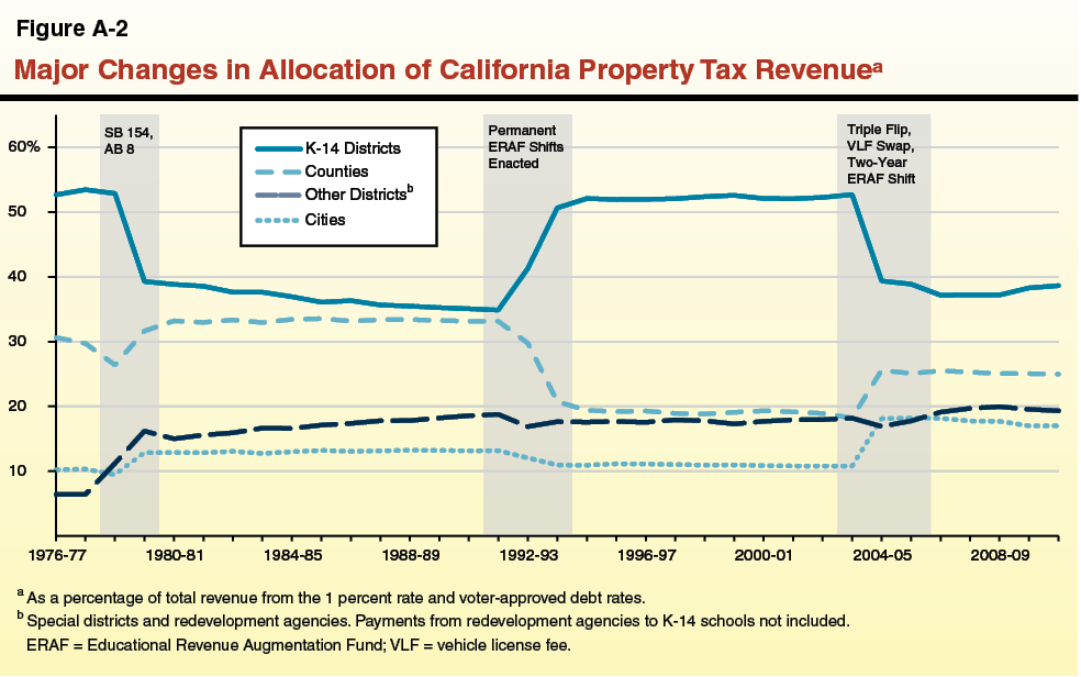
What Are “Negative Bailout Counties?”
Assembly Bill 8 did not provide additional property tax revenue to six counties (Alpine, Lassen, Mariposa, Plumas, Stanislaus, and Trinity). Under the provisions of AB 8, the increased share of the base property tax allocation to counties was calculated as the value of the SB 154 block grant plus a small adjustment for the cost of the Aid to Families with Dependent Children program less the amount of the indigent health block grant. In these six counties, the value of the indigent health block grant was so great that it exceeded the value of the adjusted SB 154 block grant. In order for these counties to be treated in the same way as all other counties, the amount of property taxes allocated to these counties was reduced. Because these counties received a smaller percentage of total property taxes collected after implementation of AB 8 relative to their pre–Proposition 13 shares, these counties are termed negative bailout counties.
New Method for Allocating Property Tax Growth. Assembly Bill 8 also established a new process for allocating growth (or decline) in property tax revenue in future years. In contrast to the property tax allocation process in 1978–79 and 1979–80 (that distributed revenue on a countywide basis without regard to where the property was located), the legislation specified that future growth in property tax revenue would be allocated only to those local governments serving the property where the revenue increase took place. Accordingly, beginning in 1980–81, AB 8 required that each local government receives the same amount of property tax it received in the prior year plus its share of any growth or decline in property tax revenue that occurred in its jurisdiction.
To ensure that each local government receives the property tax growth from the properties it serves, each county is divided into tax rate areas (TRAs). Each local government represented in a TRA receives a share of the property tax growth that occurs within that TRA. As required by AB 8, county auditors developed a methodology to determine the percentage of property tax growth—known as TRA factors—to allocate to each local government in each TRA. These TRA factors were based largely on the 1979–80 base allocation established by AB 8 (including the shift of property tax revenue from K–14 districts to other local governments). In most counties, these TRA factors remain constant. Thus, if a city received 25 percent of the property tax revenue growth generated in a TRA in 1980–81 (the first year TRA factors were used to distribute property tax revenue growth), it continued to receive 25 percent of the growth in property taxes in future years. As a result, the distribution of property tax revenue among local governments continued to closely resemble the 1979–80 distribution until the first major changes to the AB 8 system occurred in the 1990s.
In summary, the AB 8 property tax allocation system provides each local government with the same amount of property tax revenue it received in the prior year (the base), plus its share of any growth or decline in property tax revenue that occurred in its jurisdiction in the current year.
Changes to the AB 8 System
The state property tax allocation system set up in AB 8 continues to be the basis for property tax allocation among local governments today. Since 1979, however, there have been some significant changes to the original property tax allocation system contained in AB 8. In most cases, the changes reflect the complex fiscal relationship between the state and local governments. Because of the state’s role in allocating property tax revenue after Proposition 13 and in funding K–14 districts and other local programs, decisions regarding the state budget and other policy issues have led the Legislature and Governor to occasionally change how property tax revenue is distributed. We highlight the major changes in property tax allocation below. It is important to note, however, that these changes in property tax allocation do not explain the entire scope of the state–local fiscal relationship—a relationship that also has involved the realignment of many government programs and changes in other revenue sources such as the sales tax and the vehicle license fee (VLF). Some of these decisions have benefited the state fiscally, and others have benefited local governments or taxpayers.
No and Low Property Tax Cities
One change in property tax allocation relates to so–called “no and low property tax cities.” Cities that did not levy a property tax, levied only a very low property tax, or were not incorporated as cities prior to the passage of Proposition 13 typically received few property taxes under AB 8. During the 1980s the Legislature directed county auditors to modestly increase the amount of property taxes going to some of these cities by shifting a share of county property tax revenue to them.
Property Taxes Shifted to Schools
Ongoing Property Tax Shifts Started in 1990s. In 1992–93 and 1993–94, in response to serious budgetary shortfalls, the Legislature and Governor permanently redirected almost one–fifth of statewide property tax revenue—over $3 billion in 1993–94—from cities, counties, and special districts to K–14 districts. (The legislation also temporarily required redevelopment agencies to make payments to K–14 districts.) Under the changes in property tax allocation laws, the redirected property tax revenue is deposited into a countywide fund for schools, the Educational Revenue Augmentation Fund (ERAF). The property tax revenue from ERAF is distributed to non–basic aid schools and community colleges, reducing the state’s funding obligation for K–14 school districts.
The amount transferred into ERAF from each city, county, and special district was based on many factors, including the magnitude of the fiscal relief that the state provided the local government in AB 8 and, for counties, the level of taxable sales within its borders. As a result, individual local government ERAF obligations varied widely. For example, the ERAF shifts from cities formed after 1978 typically were lower than those for older cities because the newer cities did not receive any AB 8 benefits. Similarly, counties with many retail developments typically had larger ERAF shifts than rural counties because the state anticipated that extensively developed counties would receive more relief from the state’s primary ERAF mitigation measure: a half–cent sales tax for local public safety (Proposition 172, 1993). As shown in Figure A–2, after the ERAF transfer of the early 1990s, schools and community colleges once again received more than 50 percent of the state’s property tax revenue, while other local governments received less.
“Excess ERAF” Shifted Back. In the late 1990s, some county auditors reported that their ERAF accounts had more revenue than necessary to offset all state aid to non–basic aid K–14 districts. In response, the Legislature enacted a law requiring that some of these surplus funds be used for countywide special education programs and the remaining funds be returned to cities, counties, and special districts in proportion to the amount of property taxes that they contributed to ERAF. The ERAF funds that are returned to non–education local governments are known as excess ERAF.
Additional Temporary Property Tax Shift. The 2004–05 budget package also shifted $1.3 billion of property taxes from noneducation local agencies (cities, counties, special districts, and redevelopment agencies) to ERAF in 2004–05 and again in 2005–06. This temporary ERAF shift reduced the state’s funding responsibilities for K–14 districts to help address the budget shortfalls in those two years.
Changes to ERAF
The Triple Flip. In 2004, state voters approved Proposition 57, a deficit–financing bond to address the state’s budget shortfall. The state enacted a three–step approach—commonly referred to as the triple flip—that provides a dedicated funding source to repay the deficit bonds:
- Beginning in 2004–05, one–quarter cent of the local sales tax is used to repay the deficit–financing bond.
- During the time these bonds are outstanding, city and county revenue losses from the diverted local sales tax are replaced on a dollar–for–dollar basis with property taxes shifted from ERAF.
- The K–14 tax losses from the redirection of ERAF to cities and counties, in turn, are offset by increased state aid.
The triple flip increases the amount of property tax revenue going to cities and counties and reduces the amount of ERAF provided to K–14 districts. Overall, however, cities, counties, and K–14 districts do not experience any net change in revenue from the triple flip. Cities and counties receive more property tax revenue, but this revenue gain is offset by the reduction in sales tax revenue. K–14 districts receive less property tax revenue, but this is offset with increased state aid. The flip of sales taxes for property taxes ends after the deficit–financing bonds are repaid (currently estimated to occur in 2016).
The VLF Swap. The VLF—a tax on vehicle ownership—provides revenue to local governments. In 1999, the state began reducing the VLF rate and backfilling city and county revenue losses from this tax reduction with state aid. The 2004–05 budget package permanently replaced the state VLF backfill by diverting property tax revenue from ERAF and, if necessary, non–basic aid K–14 districts to cities and counties. In 2004–05, cities and counties did not experience a change in overall revenue from the VLF swap, as the amount of property tax shifted to them was equal to the VLF backfill amount. In subsequent years, state law specifies that each local government’s VLF swap payment grows based on the annual change in its assessed valuation. As a result, most cities and counties benefit fiscally from the VLF swap because assessed valuation typically grows more quickly than VLF revenue. Similar to the triple flip, K–14 districts’ property tax revenue losses are made up with increased state aid.
Distributing ERAF
The triple flip and VLF swap further expanded the use of ERAF and changed the priorities governing how its resources are used. As shown in Figure A–3, the original purpose of ERAF was to supplement the property tax revenue of non–basic aid K–14 districts. Under current law, however, funding K–14 districts falls to the fourth priority. As a result, non–basic aid school districts do not receive any ERAF resources unless additional funds remain after the county auditor (1) returns excess ERAF, (2) reimburses the triple flip, and (3) make payments for the VLF swap. This change in priorities has a significant effect on the amount of ERAF available for school districts. In 2010–11, for example, auditors in 33 counties reported using all ERAF resources for the first three priorities, leaving no ERAF for schools.
Figure A–3
Uses of ERAF Listed in Priority Order
|
Priority
|
Early 1990s
|
Late 1990s to 2004
|
2004 to Present
|
|
First
|
Fund non–basic aid K–14 districts
|
Return excess ERAF
|
Return excess ERAF
|
|
Second
|
|
Fund non–basic aid K–14 districts
|
Reimburse triple flip
|
|
Third
|
|
|
Make payments for VLF swap
|
|
Fourth
|
|
|
Fund non–basic aid K–14 districts
|
Figure A–4 displays the complex process county auditors follow to allocate ERAF and to reimburse cities and counties for the triple flip and VLF swap. This figure also shows that, under certain circumstances, it is possible that the auditor could determine that there are not enough funds to fully compensate cities and the county for the triple flip and/or the VLF swap. These funding insufficiencies are referred to as “insufficient ERAF.”
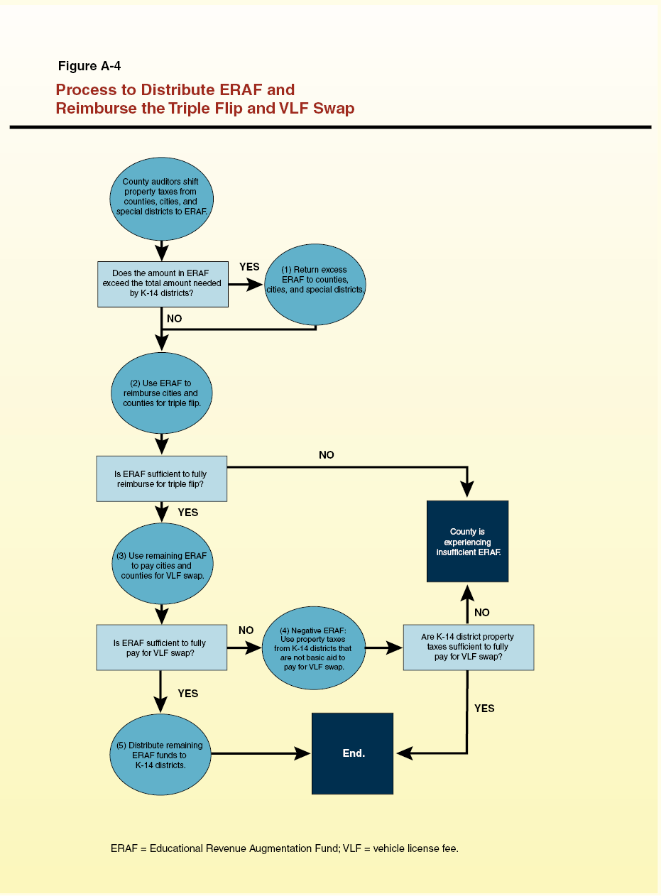
Step 1: Return Excess ERAF. As shown in the figure, the first step is for each county auditor to determine whether the funds deposited into the countywide account exceed the amount needed by all non–basic aid K–14 districts in the county, plus a specified amount for special education. If so, the excess ERAF is returned to cities, special districts, and the county in proportion to the amount of property taxes they contributed to ERAF. This calculation of excess ERAF was modified recently to reflect the increased revenue that K–14 districts and ERAF receive from the dissolution of redevelopment agencies. Specifically, to maximize the state fiscal benefit related to redevelopment dissolution, Chapter 26, Statues of 2012 (AB 1484, Committee on Budget) directs county auditors to exclude property taxes related to the dissolution of redevelopment agencies in the calculation of excess ERAF.
Step 2: Reimburse Triple Flip. Following the calculation and distribution of excess ERAF, state law directs county auditors to reimburse local governments for their revenue losses associated with the triple flip. This reimbursement is shown in the figure as step two. If the county auditor uses all available ERAF, but determines that the local governments have not been fully reimbursed for the triple flip, the county has insufficient ERAF. In this situation, additional state action is required if cities and counties are to be fully reimbursed for the triple flip.
Steps 3 and 4: Pay for VLF Swap. After reimbursing the triple flip, the next use of ERAF is to make payments to local governments for the VLF swap. If the county auditor determines that ERAF resources are not sufficient to fully pay cities and the county for the VLF swap, the county auditor redirects some property taxes from non–basic aid K–14 districts for this purpose, as shown in step 4. The redirection of school property taxes is commonly referred to as negative ERAF because it decreases K–14 property taxes rather than supplementing them (the original purpose of ERAF). If the amount of property taxes deposited in ERAF and allocated to non–basic aid school district is not enough to make the payments required under the VLF swap, then the county has insufficient ERAF. In this situation, additional state action is required for cities and counties to receive the full VLF swap payment. In 2012–13, the first time this issue came before the Legislature, the state included $1.5 million in the budget to compensate the county and cities in Amador County for insufficient ERAF.
Step 5: Distribute Remaining ERAF to K–14 Districts. Any funds remaining in ERAF after the other uses have been satisfied are distributed to schools and offset state education spending.
Limits on the State’s Authority Over Property Tax Allocation
The state’s use of property tax shifts to help resolve its severe budget difficulties—as well as other actions affecting the state–local fiscal relationship—have been a source of considerable friction between state and local government. In response, local government advocates have sponsored initiatives to limit the state’s authority over local finances, including two constitutional measures reducing the state’s authority over property tax allocation. As a result, much of the authority granted to the state in Proposition 13 and used to establish AB 8, ERAF, the VLF swap, and the triple flip is now restricted.
Proposition 1A (2004)
In 2004, voters approved Proposition 1A, amending the State Constitution to prohibit the state from shifting property tax revenue from cities, counties, and special districts to K–14 districts. The measure, however, provided an exception to its restrictions. Beginning in 2008–09, the measure allowed the state to shift a limited amount of local property tax revenue to schools and community colleges provided that the state repaid local governments for their property tax losses, with interest, within three years. The measure also specified that any change in how property tax revenue is shared among cities, counties, and special districts must be approved by two–thirds of both houses of the Legislature (instead of by majority vote). For example, state actions that shift a share of property tax revenue from one local special district to another, or from the county to a city, require approval by two–thirds of both houses of the Legislature.
The state utilized Proposition 1A’s exception for shifting property tax revenue to provide state fiscal relief in its 2009–10 budget package. Specifically, the state borrowed $1.9 billion of property tax revenue from cities, counties, and special districts—revenue equal to roughly 8 percent of each local agency’s property tax revenue. (Under Proposition 1A, the state was required to repay these funds by 2012–13. Companion legislation, however, allowed local governments to borrow against the state’s future repayments so that local government budgets were not negatively affected in 2009–10.) The 2009–10 budget package also required redevelopment agencies to make payments totaling $1.7 billion (2009–10) and $350 million (2010–11) to K–12 school districts serving students living in or near their redevelopment areas. Unlike the borrowing from cities, counties, and special districts, the state did not reimburse redevelopment agencies for these required payments.
Proposition 22 (2010)
In 2010, voters approved Proposition 22, which, among other things, prohibits the state from redirecting property tax revenue as it did in 2009–10. Specifically, Proposition 22 eliminates the state’s authority to borrow property tax revenue from local governments as previously allowed under Proposition 1A and prohibits the state from requiring redevelopment agencies to shift revenue to K–14 districts or other agencies. As discussed in the nearby box, the prohibition on shifting redevelopment funds contributed indirectly to the dissolution of redevelopment agencies in February 2012.
Proposition 1A and Proposition 22 limit the state’s authority to change property tax allocation laws. Measures that reallocate property tax revenue among counties, cities, and special districts require a two–thirds vote of the Legislature and measures that change state laws to increase the percentage of property taxes allocated to schools are prohibited. Even without additional legislative action, however, the distribution of property tax revenue will change in the near future for two reasons.
Discusses the role of property tax agents in appealing property assessments.
Examines the problems in the current property tax allocation system and discusses the tensions and trade–offs inherent in five reform proposals.
Explains the mechanics of the Educational Revenue Augmentation Fund shift and the formulas which implemented it.
Provides a timeline summarizing major changes in the state–local relationship.
Addresses some common questions about the Chapter 9 process for local governments.
Reviews the history of redevelopment agencies, the events that led to their dissolution, and the process communities are using to resolve their financial obligations.
Examines the Governor’s proposal to end redevelopment.
Discusses key events and measures that influenced state–local relations.
Summarizes key issues related to local government.
Examines the constitutional requirements related to property assessments and fees.