California’s High Housing Costs: Causes and Consequences

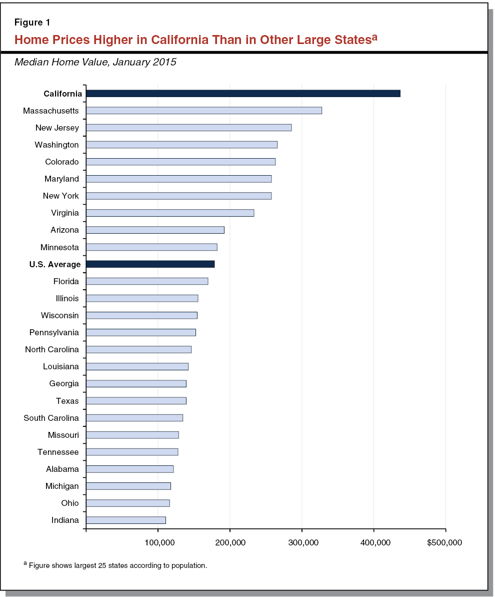
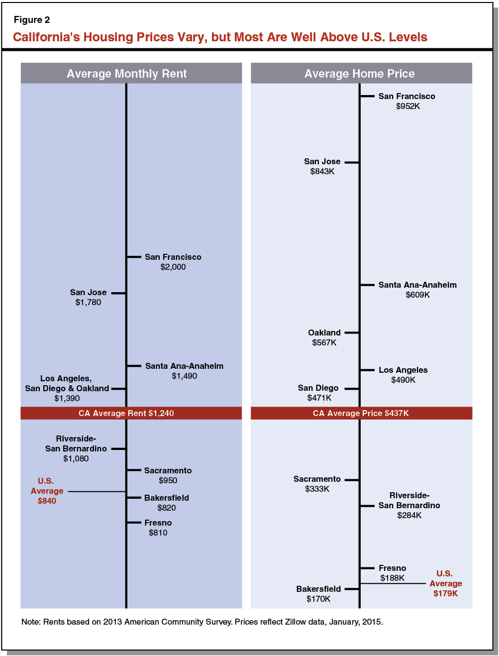
Home Prices and Rents Vary Widely Within California. In a state as large and economically diverse as California, some areas have much higher home prices and rents (and other areas much lower) than the statewide average. As shown in Figure 2, for example, home prices in California’s most expensive metropolitan area (or “metro”), San Francisco, are more than double the state average and about six times higher than Bakersfield, the state’s least expensive metro. (Throughout our report we use the U.S. census definitions of metropolitan areas—or metros. Census metros are comprised of counties—or, in some cases, a single county—that share similar socio–economic characteristics and surround a common urban core.) Rents vary throughout the state as well. The average monthly rent for a two–bedroom apartment in San Francisco ($2,000) was two and a half times greater than the average in Fresno or Bakersfield (both about $800).

Even California’s Least Expensive Housing Markets Are More Expensive Than Average. Single–family home prices and apartment rents in less costly areas of the state, such as Fresno and Bakersfield, though considered inexpensive by California standards, are about average compared with the rest of the country. Each of the state’s other major metros are well–above the rest of nation, even California’s other major inland metros, Riverside–San Bernardino and Sacramento.

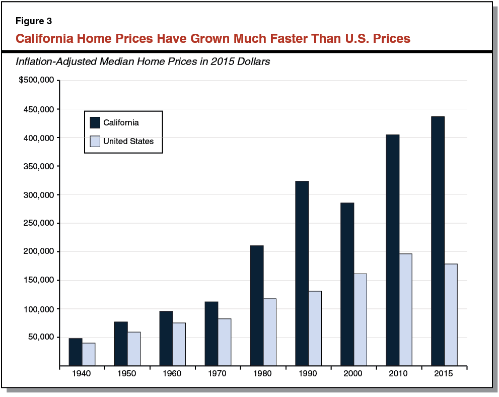
California’s Home Prices and Rents Have Risen Faster Than U.S. Average Since the 1940s. Figure 3 shows how average U.S. and California home prices have changed over time. In 1940, the average California home cost about 20 percent more than the average U.S. home. By the end of the 1940s, the state’s home prices were 30 percent higher than average. Over the next 20 years—1950 through 1970—California home prices increased about as quickly as the national average. Beginning in about 1970, however, home prices throughout the state began to accelerate. Prices were 80 percent above U.S. levels by 1980, and by 2010, the typical California home was twice as expensive as the typical U.S. home. As of 2015, average California home prices were two–and–a–half times higher than average national home prices.

Many Households Have Difficulty Affording Housing in California. As we describe in more detail later in this report, California’s high housing costs force many households to make serious trade–offs. In most instances, these trade–offs are particularly challenging for households with low incomes. Notable and widespread trade–offs include (1) spending a greater share of their income on housing, (2) postponing or foregoing homeownership, (3) living in more crowded housing, (4) commuting further to work each day, and (5) in some cases, choosing to work and live elsewhere.

Government Housing Programs Ease Housing Costs for Some. Federal, state, and local government housing programs generally work in one of two ways, by: (1) increasing the supply of moderately priced housing or (2) reducing housing costs for some households.

• Programs That Build New Housing. Federal, state, and local governments provide direct financial assistance—typically tax credits, grants, or low–cost loans—to housing developers for the construction of new rental housing. In exchange, developers reserve these units for lower–income households. (Until recently, local redevelopment agencies also provided this type of financial assistance.) Data suggests these programs together have subsidized the new construction of about 7,000 rental units annually in the state—or about 5 percent of total public and private housing construction—since the mid–1980s. In addition to direct subsidies, some local governments increase the supply of affordable housing by requiring developers of market–rate housing to set aside some of the units they are building for low– and moderate–income households, a policy called “inclusionary housing.”
• Programs That Help Households Afford Housing. In addition to constructing new housing, governments have also taken steps to make existing housing more affordable. In some cases, the federal government makes payments to landlords—known as housing vouchers—on behalf of low–income tenants for a portion of a rental unit’s monthly cost. About 400,000 California households receive this type of housing assistance. In other cases, local governments limit how much landlords can increase rents each year for existing tenants. About 15 California cities have these so–called rent controls, including Los Angeles, San Francisco, San Jose, and Oakland.

Why Is Housing Expensive in California?

A collection of factors drive California’s high cost of housing. First and foremost, far less housing has been built in California’s coastal areas than people demand. As a result, households bid up the cost of housing in coastal regions. In addition, some of the unmet demand to live in coastal areas spills over into inland California, driving up prices there too. Second, land in California’s coastal areas is expensive. Homebuilders typically respond to high land costs by building more housing units on each plot of land they develop, effectively spreading the high land costs among more units. In California’s coastal metros, however, this response has been limited, meaning higher land costs have translated more directly into higher housing costs. Finally, builders’ costs—for labor, required building materials, and government fees—are higher in California than in other states. While these higher building costs contribute to higher prices throughout the state, building costs appear to play a smaller role in explaining high housing costs in coastal areas. This section describes how each of these factors increase home prices and rents in California.

Building Less Housing Than People Demand Drives High Housing Costs

California Is Building Too Little Housing in Coastal Areas. California is a very desirable place to live, with temperate weather, long stretches of coastline, and highly educated and culturally diverse economic centers. Many households wish to live in California. However, some of California’s most sought after locations—its major coastal metros (Los Angeles, Oakland, San Diego, San Francisco, San Jose, and Santa Ana–Anaheim), where around two–thirds of Californians live—do not have sufficient housing to accommodate all of the households that want to live here. The lack of housing on the California coast means households wishing to live there compete for limited housing. This competition bids up housing costs.

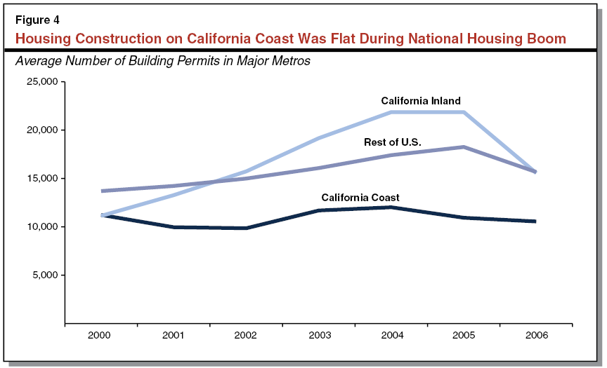
Rising home prices and rents are a signal that more households would like to live in an area than there is housing to accommodate them. Housing developers typically respond to this excess demand by building additional housing. This does not appear to be true, however, in California’s coastal metros. Building activity during the recent housing boom demonstrates this. During the mid–2000s, housing prices were rising throughout the country and, in most locations, developers responded with additional building. As Figure 4 shows, however, new housing construction, as measured by building permits issued by local officials, remained flat in California’s coastal metros. We also find that building activity in California’s coastal metros has been significantly lower than in metros outside of California that have similar desirable characteristics—such as temperate weather, coastal proximity, and economic growth—and, therefore, likely have similar demand for housing. For example, Seattle—a coastal metro with economic characteristics and average temperatures that are similar to California’s Bay Area metros—added new housing units at about twice the rate as San Francisco and San Jose over the last two decades. (Specifically, Seattle’s housing stock—its total number of housing units—grew at an average annual rate of 1.4 percent per year while San Francisco and San Jose’s housing stock grew by only 0.7 percent per year.)

Between 1980 and 2010, construction of new housing units in California’s coastal metros was low by national and historical standards. During this 30–year period, the number of housing units in the typical U.S. metro grew by 54 percent, compared with 32 percent for the state’s coastal metros. Home building was even slower in Los Angeles and San Francisco, where the housing stock grew by only around 20 percent. As Figure 5 shows, this rate of housing growth along the state’s coast also is low by California historical standards. During an earlier 30–year period (1940 to 1970), the number of housing units in California’s coastal metros grew by 200 percent.

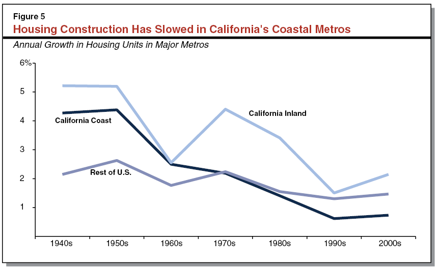
Jump in California Housing Costs Occurred as Building Slowed. A look at housing costs in California’s coastal metros in recent decades shows a connection between the slow rate of building and higher housing costs. The slowdown in building in California’s coastal metros corresponded with a substantial rise in housing costs relative to the rest of the country. In 1970, home prices in the state’s coastal metros were about 50 percent more expensive than in the rest of the country. This gap has widened considerably since that time. Homes in the coastal metros are now more than three times more expensive than the rest of the country. Similarly, rents have grown more expensive, with the gap between the coastal metros and the rest of the country increasing threefold since 1970 (from 16 percent more expensive to around 50 percent more expensive).

Link Between Development and Housing Costs Exists Elsewhere Too. The same relationship between growth of housing supply and housing costs exists throughout the country, suggesting that what has occurred in California is not coincidental. Looking broadly at major metropolitan counties (counties comprising metros with a population of 500,000 or greater) throughout the country, places with slower housing growth generally have more expensive housing. Based on U.S. Census data, the median home price in 2010 was just over $300,000 in the fifth of counties that grew the slowest between 1980–2010, compared with $195,000 in the fifth of counties that grew the fastest.

Our review indicates that that the relationship between growth of housing supply and increased housing costs is complex and affected by other factors—such as demographics, local economies, and weather. Nonetheless, using common statistical techniques to account for the influence of these other factors, there remains a strong relationship between home building and prices. For example, our analysis suggests that—after controlling for other factors—if a county with a home building rate in the bottom fifth of all counties during the 2000s had instead been among the top fifth, its median home price in 2010 would have been roughly 25 percent lower. Similarly, its median rent would have been roughly 10 percent lower.

Spillover of Demand to Live on the Coast Affects Housing Costs in Inland California. In contrast to the coast, more home building has occurred in California’s inland metros (Bakersfield, Fresno, Riverside–San Bernardino, and Sacramento) than typical U.S. metros. California’s inland metros added housing at about twice the rate of the typical U.S. metro between 1980 and 2010. Yet housing costs in much of inland California are above average relative to the rest of the country. High housing costs in the state’s inland metros appear to result largely from their proximity to California’s coast. Some households and businesses that want to locate on California’s coast but find housing too expensive there locate in California’s inland metros instead. This displaced demand places pressure on inland housing markets and results in higher home prices and rents there. Examining the relationship between housing costs in neighboring counties throughout the country using U.S. Census data from 1980 and 2010, we find that this spillover effect is substantial. Our analysis suggests that—after accounting for a variety of other factors that can affect housing costs—a 10 percent increase in housing costs in a county is associated with a roughly 5 percent increase in housing costs in its neighboring counties.

High Land Costs and Low Density Development Make Housing Expensive

Land Costs Are High on the California Coast. Land prices on the California coast are among the highest in the country. In contrast, land prices in inland California typically are at or below the national average. Comparing land prices across metropolitan areas can be difficult, largely due to data limitations. Nonetheless, several estimates of land values are available in the economics literature and they find that land is considerably more expensive on California’s coast. One analysis of land sales between 2005 and 2010 found that land prices in California’s metros ranged from twice as expensive as the average U.S. metro (Oakland and San Diego) to more than four times as expensive (San Francisco). We also examined existing data to better understand the value of single–family home lots in different areas. Using American Housing Survey data from 2011, we found an even greater divergence between California and the rest of the country. Residential land in an average U.S. metro was valued at around $20,000 per acre, compared with over $150,000 in California’s coastal metros. Land values were highest in San Francisco, where an acre of land was valued at nearly $400,000.

High Land Costs Can Be Offset Through Dense Development. Although high land costs can translate into higher home prices and rents, it is possible to offset the effects of high land costs through more dense development. (The density of housing refers to the number of housing units per unit of land—typically measured in units per acre. Higher–density housing, such as an apartment building, has more housing units per acre.) Building more units on the same plot of land allows a developer to spread land costs across more units, lessening the impact of land costs on the cost of each unit. This is because land costs are fixed and do not increase if a developer builds additional units. For example, if a developer builds five homes on a plot of land that costs $100,000, the land cost per unit is $20,000. Alternatively, if the developer builds ten homes on the same plot of land, the land cost per unit is only $10,000. Builders faced with high land costs, therefore, generally will build more dense housing. When this occurs, the effect of high land costs on home prices and rents is reduced.

Little Increase in Housing Densities in Coastal Metros. While developers typically respond to high land costs by building more dense housing, this response appears to be somewhat limited in most of California’s coastal metros. As a result, high land costs in these areas have translated more directly into higher housing costs. We examined U.S. Census data to compare changes in housing densities during the 2000s in California’s coastal metros to changes in metros elsewhere in the country. Our initial review of California’s coastal metros found that housing densities rose significantly faster in San Francisco than the other California coastal metros, which is unsurprising given that San Francisco’s land prices are higher than just about anywhere else in the U.S. Because San Francisco appeared to be exceptional, we focused the rest of our review on California’s other coastal metros. We compared changes in density in these other California coastal metros with metros that have land prices and existing housing densities similar to those found on California’s coast. We selected Boston, Las Vegas, Miami, Seattle, and Washington D.C. as our comparison group of metros. Our review found that, during the 2000s, the housing density of a typical neighborhood in California’s coastal metros rose by 4 percent. This increase in density was considerably less than the 11 percent average increase in our comparison group. Furthermore, we estimate that the new housing built in these comparison metros was about 40 percent more dense than housing built in California’s coastal metros. New housing in the comparison metros had an average density of about 14 units per acre, compared with about ten units per acre in California’s coastal metros.

Building Costs Increase Housing Costs

Building Costs Are Higher in California. Aside from the cost of land, three factors determine developers’ cost to build housing: labor, materials, and government fees. All three of these components are higher in California than in the rest of the country. Construction labor is about 20 percent more expensive in California metros than in the rest of the country. California’s building codes and standards also are considered more comprehensive and prescriptive, often requiring more expensive materials and labor. For example, the state requires builders to use higher quality building materials—such as windows, insulation, and heating and cooling systems—to achieve certain energy efficiency goals. Additionally, development fees—charges levied on builders as a condition of development—are higher in California than the rest of the country. A 2012 national survey found that the average development fee levied by California local governments (excluding water–related fees) was just over $22,000 per single–family home compared with about $6,000 per single–family home in the rest of the country. (This survey reflects school facilities fees imposed during this period and not the higher so–called “Level 3” fees that school districts may impose in the future if the State Allocation Board makes certain declarations about the availability of school construction funds.) Altogether, the cost of building a typical single–family home in California’s metros likely is between $50,000 and $75,000 higher than in the rest of the country.

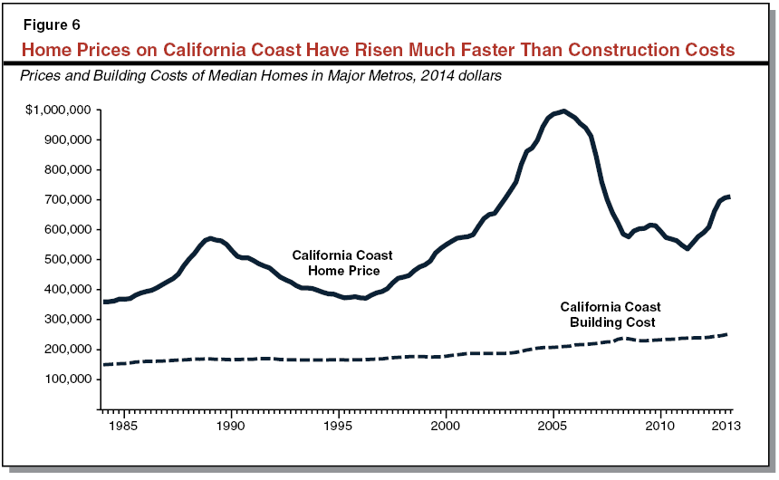
Effect of Building Costs on Prices and Rents Varies Across Regions of the State. Higher building costs contribute to higher housing costs throughout the state. The relationship between building costs and prices and rents, however, differs across inland and coastal areas of the state. In places where housing is relatively abundant, such as much of inland California, building costs generally determine housing costs. This is because landlords and home sellers compete for tenants and homebuyers. This competition benefits renters and prospective homebuyers by depressing prices and rents, keeping them close to building costs. In these types of housing markets, building costs account for the vast majority of home prices. In two major inland metros—Riverside–San Bernardino and Sacramento—building costs account for over fourth–fifths of home prices. In contrast, in coastal California, the opposite is true. Renters and home buyers compete for a limited number of apartments and homes, bidding up prices far in excess of building costs. Building costs account for around one–third of home prices in California’s coastal metros. Under these circumstances, as Figure 6 shows, building costs explain only a small portion of growth in housing costs. Instead, increasing competition for limited housing is the primary driver of housing cost growth in coastal California.

Why DO Coastal Areas Not Build Enough Housing?

As we discussed in the last section, California’s home prices and rents have risen because housing developers in California’s coastal areas have not responded to economic signals to increase the supply of housing and build housing at higher densities. A collection of factors inhibit developers from doing so. The most significant factors are:

• Community Resistance to New Housing. Local communities make most decisions about housing development. Because of the importance of cities and counties in determining development patterns, how local residents feel about new housing is important. When residents are concerned about new housing, they can use the community’s land use authority to slow or stop housing from being built or require it to be built at lower densities.
• Environmental Reviews Can Be Used to Stop or Limit Housing Development. The California Environmental Quality Act (CEQA) requires local governments to conduct a detailed review of the potential environmental effects of new housing construction (and most other types of development) prior to approving it. The information in these reports sometimes results in the city or county denying proposals to develop housing or approving fewer housing units than the developer proposed. In addition, CEQA’s complicated procedural requirements give development opponents significant opportunities to continue challenging housing projects after local governments have approved them.
• Local Finance Structure Favors Nonresidential Development. California’s local government finance structure typically gives cities and counties greater fiscal incentives to approve nonresidential development or lower density housing development. Consequently, many cities and counties have oriented their land use planning and approval processes disproportionately towards these types of developments.
• Limited Vacant Developable Land. Vacant land suitable for development in California coastal metros is extremely limited. This scarcity of land makes it more difficult for developers to find sites to build new housing.

We discuss these factors in more detail below.

Community Resistance Is Heightened

Local Communities Make Most Decisions About New Housing. Cities and counties generally decide when, where, and to what extent housing development will occur (cities make these decisions within their boundaries and counties in unincorporated areas). Local zoning laws and building codes specify where housing may be built, as well as its density, quality, and style. Housing developers are required to obtain building permits from city and county planning departments and typically must gain approval from local planning commissions and city councils or county boards of supervisors. Cities and counties also prepare General Plans that shape their communities’ long–term development patterns.

Local Resident Concerns About New Housing Are Common Throughout the U.S. In general, many potential or perceived downsides of new housing accrue to existing residents, while many of the benefits of new housing accrue to future residents. As a result, existing residents sometimes take steps to slow or stop development.

There are many possible reasons residents may be hesitant about new housing. Some residents may see new housing as a threat to their financial wellbeing. For many homeowners, their home is their most significant financial investment. Existing homeowners, therefore, may be inclined to limit new housing because they fear it will reduce the values of the homes.

Residents also may feel that new housing reduces their nonfinancial wellbeing. Many people, as they become accustomed to their lifestyle and the character of their neighborhood, naturally are hesitant about change and future unknowns. It is unsurprising then that they would be concerned about adding new housing to their community because it presents uncertainty and possibilities of change. Expanded development can strain existing infrastructure—such as streets and roads, schools, and parks—requiring residents to change the way they use these public goods. For example, new development may increase traffic on existing streets and roads, forcing some residents who commute via car to take public transportation instead. Strains on existing infrastructure also may require state and local governments to make new investments in infrastructure to expand capacity. New housing also can alter the character of a community, shifting it from a rural to an urban setting or from a traditional single–family home neighborhood to a neighborhood with a mix of densities and land uses. In addition, new housing can place strains on natural and environmental resources, in some instances making it more difficult to ensure adequate air and water quality or to protect natural ecosystems.

Opposition to New Housing Appears to Be Heightened on the California Coast. Hesitance about new housing can lead residents to pressure local officials to use their land use authority to slow or block new development or may result in residents directly intervening in land use decisions via the initiative and referendum process. Compared with the rest of the country, these types of activities appear to occur more often in California’s coastal communities, suggesting that community opposition to housing is heightened in these areas.

Many Coastal Communities Have Growth Controls. Over two–thirds of cities and counties in California’s coastal metros have adopted policies (known as growth controls) explicitly aimed at limiting housing growth. Many policies directly limit growth—for example, by capping the number of new homes that may be built in a given year or limiting building heights and densities. Other policies indirectly limit growth—for example, by requiring a supermajority of local boards to approve housing projects. Research has found that these policies have been effective at limiting growth and consequently increasing housing costs. One study of growth controls enacted by California cities found that each additional growth control policy a community added was associated with a 3 percent to 5 percent increase in home prices.

Project Reviews Along Coast Often Are Slow and Cumbersome. Cities and counties often require housing projects to go through multiple layers of review prior to approval. For example, a project may require independent review by a building department, health department, fire department, planning commission, and city council. Each layer of review can increase project approval time. Additional complexity in review processes also creates avenues for concerned residents to slow building or reduce its size and scope, as the story in the nearby box shows. One survey of city and county officials nationwide suggests that communities in California’s coastal metros take about two and a half months longer, on average, to issue a building permit than in a typical California inland community or the typical U.S. metro (seven months compared to four and a half months). Divergence from the rest of the country was more significant in some communities—for example, typical approval time was over a year in San Francisco and over eight months in the City of Los Angeles. If a project required a change in local zoning laws—as is common among large projects—approval time was much longer. The average time to approve a rezoning was just under a year in California’s coastal metros, about three months longer than in a typical California inland community or a typical U.S. metro. Researchers have linked additional review time to higher housing costs. A study of jurisdictions in the Bay Area found that each additional layer of independent review was associated with a 4 percent increase in a jurisdiction’s home prices.

Local Ballot Measures on Coast Have Limited Development. Many significant land use decisions in California’s coastal communities are made by voters. More often than not, voters in California’s coastal communities vote to limit housing development when given the option. Our review of local elections data between 1995–2011 found that voters in California’s coastal metros took a position that limited housing growth—either by voting “yes” for a measure constraining growth or voting “no” for a measure that would allow growth—about 55 percent of the time. On average, coastal communities as a whole approved five measures per year limiting housing growth (or rejected measures allowing new building). While most major local jurisdictions throughout the country have some form of an initiative and referendum process, California’s high degree of voter involvement in land use decisions appears to be unique. One review of election results across the country during the November 2000 election found that just under half of all measures related to land use planning and growth management were in California.

Why Is Community Resistance to New Housing Heightened on California Coast? A collection of factors come together on the California coast to create a particularly heightened level of community resistance to new housing. High demand to live on California’s coast results in constant pressure for additional housing. At the same time, residents of California’s coast have much at stake in decisions about housing growth, as their communities have very high home values and desirable natural amenities. As a result, residents often push back against proposals for new housing. In addition, there is very little vacant land for new housing, meaning that development often takes the form of redevelopment in established neighborhoods. Redevelopment changes these neighborhoods, creating additional concerns for existing residents.

CEQA Can Be Used to Delay or Reduce Building Activity

CEQA Requires Environmental Review for New Housing. CEQA was enacted in 1970 in order to ensure that state and local agencies consider the environmental impact of their decisions when approving a public or private project. Under CEQA, before approving new housing (or other development), cities and counties usually must conduct a preliminary analysis to determine whether a project may have significant adverse environmental impacts. If it is determined that a project might create significant impacts, then an environmental impact report (EIR) must be prepared. An EIR provides detailed information about a project’s likely effect on the environment, considers ways to mitigate significant adverse environmental effects, and examines alternatives to the project. Where an EIR finds that a project will have significant adverse environmental impacts, a city or county is prohibited from approving the project unless one of the following two conditions is met: (1) the project developer makes modifications that substantially lessen the adverse environmental effects or (2) the city or county finds that economic or other project benefits override the adverse environmental effects. This level of environmental review for private housing development is uncommon among U.S. states. Only four other states have comparable requirements.

CEQA Can Be Used to Reduce New Housing Development. The CEQA process can provide valuable information to decision makers and help to avoid unnecessary environmental impacts. The CEQA review process also provides many opportunities for opponents to raise concerns regarding a project’s potential effects on a wide array of matters, including parking, traffic, air and water quality, endangered species, and historical site preservation. A project cannot move forward until all concerns are addressed, either through mitigation or with a determination by elected officials that benefits of the project outweigh the costs. In addition, after a local governing board approves a project, opponents may file a lawsuit challenging the validity of the CEQA review. As a result of these factors, CEQA review can be time consuming for developers. Our review of CEQA documents submitted to the state by California’s ten largest cites between 2004–2013 indicates that local agencies took, on average, around two and a half years to approve housing projects that required an EIR. The CEQA process also, in some cases, results in developers reducing the size and scope of a project in response to concerns discovered during the review process.

Limited Local Government Fiscal Incentive to Approve Housing Development

Local Governments Weigh Fiscal Impacts of Land Use Decisions. When property is developed, communities usually:

• Receive Increased Tax Revenues. Many developments, for example, generate increased property and/or sales tax revenues for the communities in which they are located.
• Face Increased Demand for Public Services and Infrastructure. For example, developments can trigger increased demand for local governments to provide police and fire services to new residents or to expand streets and roads to accommodate increased vehicle traffic.

Because different types of developments yield different amounts of tax revenues and service demands, local governments throughout the nation commonly examine these fiscal effects when considering new developments or planning for future development. As a matter of fiscal prudence, development that does not generate sufficient revenues to fund a local government’s new costs often is revised or rejected.

California Communities Often Benefit More From Commercial Development. In California, cities and counties typically find that commercial developments—particularly major retail establishments, auto malls, restaurants, and hotels—yield the highest net fiscal benefits. This is because the increased sales and hotel tax revenue that a city (or, in the case of a development in an unincorporated area, the county) receives from these developments often more than offsets the local government’s costs to provide them public services. As a result, cities and counties often encourage these types of commercial developments to locate within their jurisdictions—for example by zoning large sections of land for these purposes and by offering subsidies or other benefits to the prospective business owners.

In contrast, many California cities and counties find that housing developments lead to more local costs than offsetting tax revenues. This is because these properties do not produce sales or hotel tax revenues directly and the state’s cities and counties typically receive only a small portion of the revenue collected from the property tax. In addition, lower–density luxury housing often “pencils out” more favorably from a local government standpoint than higher–density moderate cost housing. This is because the luxury housing generates higher levels of property tax revenues per new resident.

Not surprisingly given these incentives, many cities and counties have oriented their land use planning and approval process disproportionately towards the development of commercial establishments and away from higher–density multifamily housing.

Limited Developable Land

Topography Limits Developable Land. Topography is the primary constraint on developable land in California’s coastal metros. Just under two–thirds of the area surrounding the urban centers on California’s coast is undevelopable due to mountains, hills, ocean, and other water. This compares to less than a quarter of land lost due to topography in a typical U.S. metro.

More Extensive Development Has Left Limited Vacant Land. Another constraint on development in California’s coastal metros is the extent to which land already has been developed. Land in the center of California’s major metros (defined as land within a 25 mile radius of the city hall of the metro’s largest city) contains housing built at densities similar to metros in the rest of the country. By comparison, land in the outlying areas of California coastal metros (land beyond the 25 mile radius) has housing at about twice the density as outlying areas in metros elsewhere in the country (four housing units per acre in California versus about two units per acre elsewhere in the country). More development in outlying areas typically leaves less vacant land for future development.

Redeveloping Land Possible, but More Difficult and Expensive. Overall, one survey of land in California’s urban areas conducted in 2006 found that less than 1 percent of land in California’s coastal urban areas was developable and vacant. Limited vacant land, however, does not mean that development must cease. Previously developed but abandoned or underutilized parcels can be redeveloped. Older, lower–density housing can be replaced with new higher–density housing. These types of redevelopment activities can yield increased housing supply even in areas where little or no vacant land exists. Redevelopment, however, often is more cumbersome and expensive than development on vacant land. Developers must demolish old buildings and often are required to address environmental pollutants and toxic substances leftover from previous uses. New construction, therefore, is likely to proceed at a slower pace where land must be redeveloped.

Community Decisions Can Exacerbate Land Scarcity. City and county land use policies can alleviate pressures created by limited vacant land by encouraging redevelopment and allowing developers to build more housing on each parcel. In many California communities, however, for reasons discussed earlier the opposite is true. Zoning laws often require developers to build housing at densities that are common elsewhere in the community, preventing developers from building at higher densities to counter high land costs. In addition, local communities sometimes pressure developers to reduce a project’s planned density during approval processes. Cities and counties also can magnify the effect of scarce land on housing costs by choosing to allocate a large share of available land to nonhousing uses, such as retail and hotel development.

How Big Is California’s Housing Shortage?

In recent decades, California has built new housing at a slower rate than the rest of the country and much of this new housing has been built in relatively underdeveloped inland areas. As a result, California’s supply of housing has not kept pace with demand to live in the state and housing costs have grown faster than the rest of the country. To give the Legislature an estimate of the magnitude of this housing shortfall, we developed a quantitative model of California’s housing market. This section begins with a description of this model and its findings and then assesses the likelihood of similar–sized housing shortfalls continuing in the future.

Estimating California’s 1980–2010 Housing Shortage

Our Model. As described more fully in this report’s technical appendix, our model uses standard statistical tools to examine housing price and supply changes in major metropolitan counties throughout the United States and control for various factors. A key element of our model is its ability to estimate the number of housing units that needed to be built to satisfy demand and keep housing prices within certain ranges. We used the model to estimate the amount of housing that—had it been built between 1980 and 2010—would have kept California’s median housing price from growing faster than the nation’s. Under this approach, California’s median housing prices still would have grown between 1980 and 2010, but the rate of growth would have been slower and comparable to that in the rest of the country. Under this housing supply scenario, California’s housing prices would have been 80 percent higher than the U.S. median in 2010, instead of reaching twice the U.S. median (as actually occurred).

Key Findings. As we discuss further below, our model estimates that keeping California home prices from growing faster than the nation between 1980 and 2010 would have required the state to have:

• Built substantially more new housing—in the range of 70,000 to 110,000 additional units each year.
• Shifted more home building to coastal areas.
• Built denser housing, concentrated in central cities.

More Housing in Total. Between 1980 and 2010, California’s major metros added about 120,000 new housing units each year. Our analysis suggests that between 190,000 units per year and 230,000 units per year were needed to keep California’s housing cost growth in line with cost escalations elsewhere in the U.S. (Our midpoint estimate—which represents our single best guess at California’s housing need—is slightly above 210,000 units per year. For the remainder of this section, we discuss our midpoint estimates.) Figure 7 shows our estimate of additional housing construction needed in each of the past three decades. These statewide estimates, however, mask significant variation across regions of the state, as well as across cities within those regions.

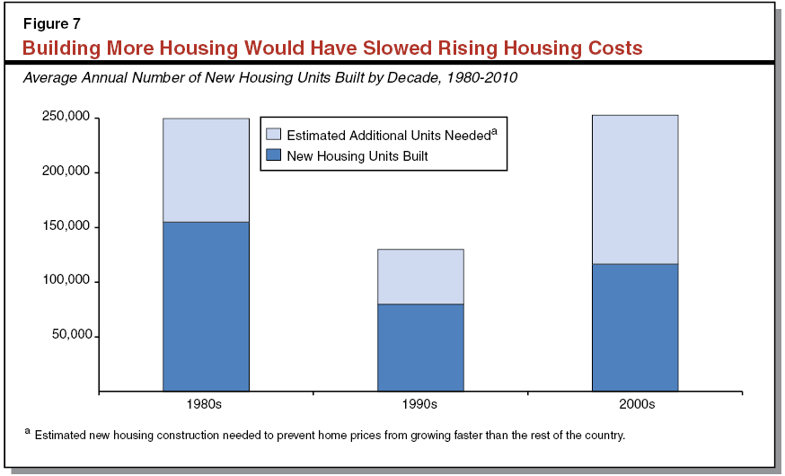
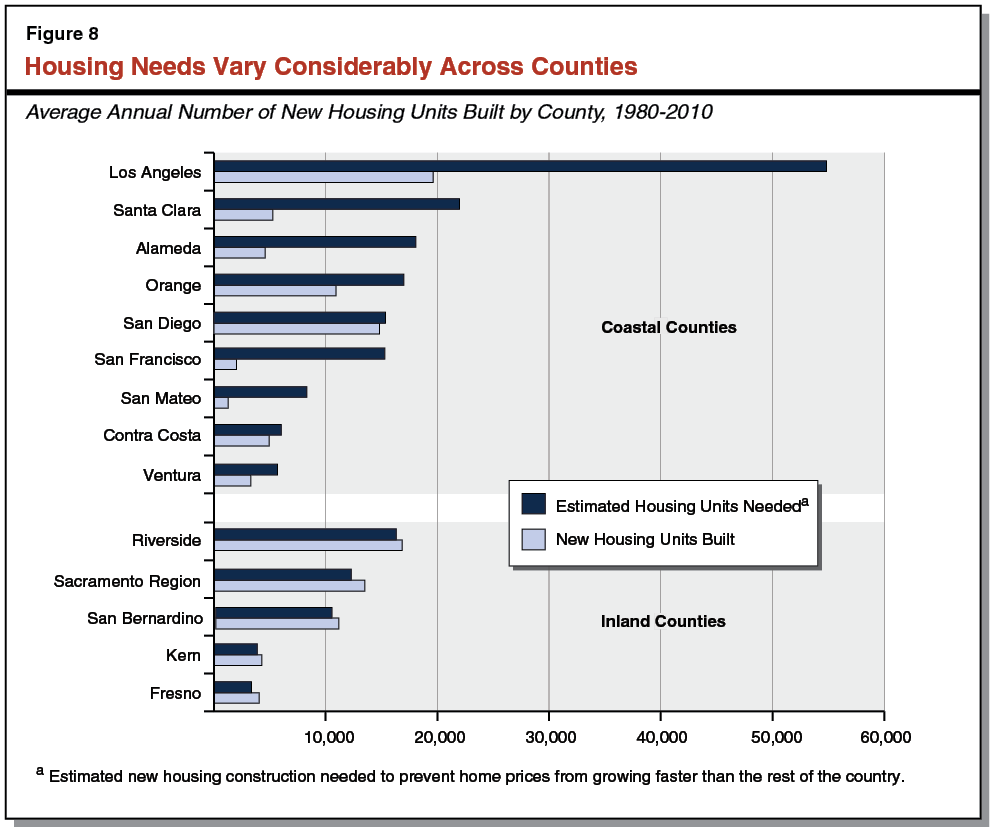
More Building on Coast, Less Inland. Our estimates suggest that, to contain price growth, the geographical distribution of new housing over the past three decades needed to be different, with significantly more building in coastal areas and somewhat less building in inland areas. Figure 7 compares actual home building in California’s largest counties between 1980 and 2010 to the levels of building that we estimate would have kept home price growth in line with the rest of the country. As Figure 8 shows, most of California’s coastal counties needed to build three times as much (or more) housing as they did, while inland counties built more housing than our estimates suggest was needed to contain price growth.

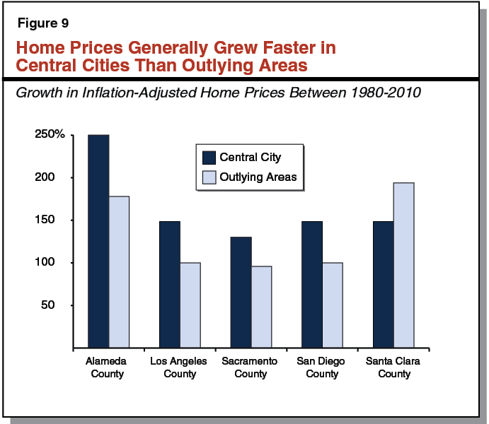
More Building in Central Cities, Less in Outlying Areas. As we discussed above, insufficient housing was built in California’s coastal counties, causing demand to spill over into inland areas. A similar situation appears to have occurred within the coastal counties. Insufficient housing was built in the central cities of coastal counties to satisfy demand for housing, driving development into suburban and rural areas. As Figure 9 shows, between 1980 and 2010, home prices in most of California’s largest cities grew faster than home prices in surrounding areas within the same county. In general, because unmet demand results in competition for housing and rising costs, home prices and rents are highest where unmet demand is greatest. These price trends, therefore, suggest that unmet demand for housing is greater in central cities relative to surrounding areas. More housing development was needed in central cities relative to surrounding areas to contain growth in housing costs.

Denser Housing. Much of the buildable land in California’s coastal metros has been developed. Because of this, adding more housing to these metros would have required housing to be built more densely. Figure 10 shows our estimates of how dense housing would be in California’s coastal metros if they had grown over the last 30 years at the rate necessary to keep their prices in line with the rest of the country. Housing densities in many coastal counties would be more than two–thirds higher under the LAO growth scenario than they are today. Despite these sizeable increases, housing densities in California’s coastal metros under our growth scenario would not be unprecedented. As Figure 10 shows, there are other metropolitan counties throughout the country that currently are as dense as California’s coastal metros would be under our growth scenario.

More Housing Would Mean More Californians. If California had added 210,000 new housing units each year over the past three decades (as opposed to 120,000), California’s population would be much greater than it is today. We estimate that around 7 million additional people would be living in California. In some areas, particularly the Bay Area, population increases would be dramatic. For example, San Francisco’s population would be more than twice as large (1.7 million people versus around 800,000). In other areas of the state, where significant housing development occurred due to spillover demand in the state’s coastal metros, population would likely be about what it is today or potentially smaller.

What Does This Estimate Tell Us About the Future?

As we have discussed, a collection of barriers have prevented California’s housing developers from responding to high demand to live on California’s coast by building more housing there. Our analysis in this section suggests that these barriers have created a major disconnect between the demand for housing and its supply. Looking forward, there are many reasons to think this dynamic will continue. Many of the primary factors that make California desirable—moderate weather, natural beauty, and coastal proximity of its major metros—are ongoing. At the same time, we see no signs that coastal community resistance to new housing construction is abating. In addition, many state and local policies that have slowed or stopped development in recent decades remain in effect today. We therefore think that, in the absence of major policy changes, California’s trend of rapidly rising housing costs is very likely to continue in the future. Our analysis suggests that building substantially more housing in coastal urban areas—possibly as much as 100,000 additional units each year—could prevent California’s housing costs from continuing to grow faster than the U.S. In our view, this major finding that demand for housing in California substantially exceeds supply should inform discussions and decision making regarding state and local government housing policies.

We do, however, recognize that any attempt to estimate the state’s future housing needs faces significant uncertainties. Unforeseeable changes in demographics, economic conditions, or technology could shift dramatically the dynamics of California’s housing markets. Readers, therefore, should focus less on our specific estimates and more on the simple story they tell: to contain rising housing costs, California would have to build significant more housing, especially in coastal urban areas.

What Are the Consequences of California’s Expensive Housing?

Housing costs are the largest component of most households’ spending. Because housing is such a large financial consideration, households make careful decisions about the location, cost, and amenities of their home. Faced with high home prices and rents, California households must decide: how much income can they spend on housing (and therefore what must they consume less of); where can they find housing of this sort; and how far is this housing from work, school, and local amenities? Each household finds its unique answers to these questions, typically responding to high housing costs with a combination of trade–offs. In the following section, we review five significant trade–offs households make when faced with high housing costs. These include: (1) spending a larger share of income on housing, (2) postponing or foregoing homeownership, (3) living in more crowded housing, (4) commuting further to work each day, or (5) sometimes, choosing to work and live elsewhere. We also discuss how these serious trade–offs affect the state’s economy.

Households Spend More of Their Income on Housing

Housing Costs Are a Major Consideration for Most Households. Housing costs are the largest component of most household’s spending each month. For homeowners, these costs include monthly principal and interests payments; property taxes and homeowner’s insurance; and household utilities like water, gas, and electricity. For renters, housing costs are their monthly rent and any utilities the tenant pays. On average, American households spend about one–quarter of their gross monthly income on housing. (More information on this data is available in the box below.)

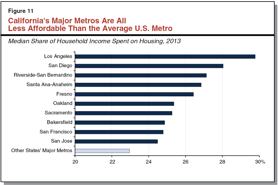
Despite Relatively Higher Incomes, Californians Devote Larger Share to Housing. Median household income in California is about $9,000 more annually than the national median. Median California housing costs, however, are about $5,300 greater as well. For most California households, therefore, higher housing costs consume a large portion of their higher income. Specifically, the median California household spends about 27 percent of their monthly income on housing. The median household in the rest of the country, on the other hand, spends about 23 percent. This above–average trend exists throughout California. As shown in Figure 11, households in each of the state’s major metros spend an above–average share of their income on housing. In the state’s largest metro, Los Angeles, the average household spends 30 percent of their income on housing, 7 percent more than the national average.

The figures discussed above are median housing costs as a share of income; that is, the amount of income spent on housing where one–half of households spend a smaller share and one–half spend a larger share. In this way, they best reflect the typical household’s experience. For other types of households, however, differences between Californians and the rest of the country may be more or less pronounced.

Low–Income Californians Spend Greater Share of Income on Housing. Households with low incomes spend a smaller amount of money each month on housing than do households with higher incomes. Lower–income households nevertheless spend a much larger share of their total income on housing, leaving fewer resources leftover for other spending and savings priorities. As shown in Figure 12, California households in the bottom quarter of the income distribution—the poorest 25 percent of households—report spending four times more of their income (67 percent, on average) than households in the top quarter of the income distribution (16 percent, on average).

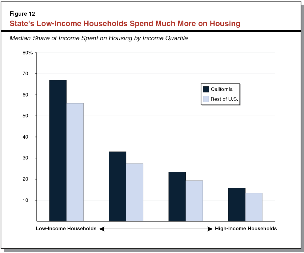
Gap Between California and U.S. Largest for Low–Income Households. The difference between what California households spend and what U.S. households typically spend—a difference that is the byproduct of the state’s high housing costs—is largest for low–income households and smallest for upper–income households. As shown in Figure 12, California households with incomes in the bottom quartile report spending 67 percent of their income on housing, about 11 percent more than low–income households elsewhere. This “gap” persists across most income groups but becomes smaller as income increases. For higher–income households, as shown in the figure, California households and households in other areas spend a similar, much smaller, share of their income on housing. These findings suggest that California’s high housing costs are particularly challenging for the state’s low–income households.

Renters Spend a Much Larger Share of Income on Housing. Nationwide, renter households spend a significantly larger share of their income on housing. The median renter spends about 30 percent of his or her income on housing, whereas the median homeowner spends 20 percent. Primarily, this occurs because renter households have notably lower incomes, on average, than owner households. In addition to generally lower income levels, renters spend more on housing, on average, because a portion of homeowners have owned their homes for many years and therefore have very low monthly mortgage costs or no mortgage costs whatsoever.

Low–Income Households That Spend More on Housing Spend Less on Essentials. In high cost areas, households typically spend a larger share of their income on housing. As a result, households have less money available for other types of spending. For households with above–average incomes, higher housing costs may mean they spend less on other items, but these households typically have sufficient resources to purchase regular household necessities. For low–income households, though, high housing costs cut into spending considered more necessary. According to Harvard’s Joint Center for Housing Studies, low–income households who spent more than half of their income on housing spent 39 percent less on food than other low–income households that spent less than half their income on housing.

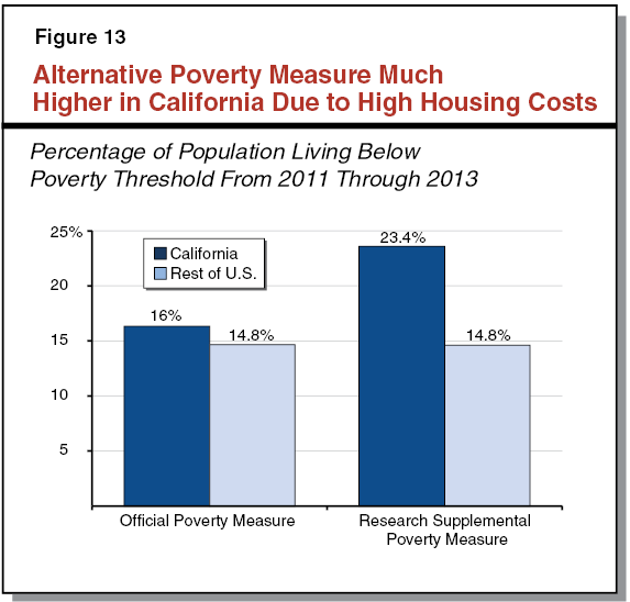
High Housing Costs Contribute to Poverty in California. The federal government each year calculates what share of each state’s population lives in poverty. Typically, poverty is calculated by the Official Poverty Measure, which defines a family as poor if their pretax cash income is less than a poverty threshold that is standard across the nation. Based on this measure, California’s poverty rate is slightly higher than the rest of the United States, as shown in Figure 13. The federal government also reports poverty levels using an alternative measure, the so–called Supplemental Poverty Measure, which adjusts poverty thresholds based on local costs of living. Primarily because of California’s high housing costs, the state’s alternative poverty level is 23.4 percent, the highest in the nation and almost 9 percentage points higher than average.

High Housing Costs May Make Personal Finances More Fragile. One byproduct of spending a large share of one’s income on housing is that personal finances may be more fragile—meaning a smaller share of a household’s income is available for nonhousing goods and services, including savings. As a result, these households may find it more difficult to accommodate a drop in household income because they have a smaller amount of nonhousing disposable income and likely have smaller available savings.

Fewer Households Own Their Homes

Homeownership Helps Households Build Wealth. The federal government has actively promoted homeownership since it restructured the housing finance system during the Great Depression. As a result, beginning in 1940s, the U.S. homeownership rate rose steadily and substantially, peaking at 70 percent just before the recent housing crisis. (Since then, it has fallen 64 percent, a low not seen since the 1990s.) Homeownership helps households build wealth, requiring them to amass assets over time. Among homeowners, saving is automatic: every month, part of the mortgage payment reduces the total amount owed and thus becomes the homeowner’s equity. For renters, savings requires voluntarily foregoing near–term spending. Due to this and other economic factors, renter median net worth totaled $5,400 in 2013, a small fraction of the $195,400 median homeowner’s net worth. For many households in high housing cost areas, though, homeownership’s benefits remain out of reach, as higher home prices (relative to area incomes) mean fewer and fewer households can afford to become homeowners.

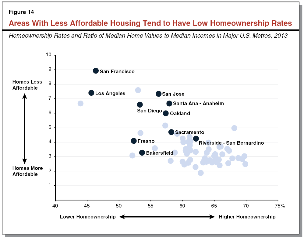
California’s Homeownership Rate Among Lowest in Nation. About 64 percent of U.S. households own their homes, but only 54 percent of California households do. (Only New York State and Nevada have lower homeownership rates.) In areas with high housing prices, including those in California, homeownership tends to lag behind more affordable areas. Figure 14 shows that, across the country, metro areas where home prices are high relative to average income levels tend to have lower homeownership rates. Most of California’s major metros, and all of California’s coastal metros, fall into this category.

Households That Do Buy Purchase Later and Take on More Debt. An additional byproduct of higher home prices is that young people delay purchasing their first home, possibly because saving for a down payment takes longer or households are not able to generate qualifying income levels until later in their careers. According to National Association of Realtors data, the median first–time homebuyer in California in 2013 was 34 years old, three years older than the median first–time homebuyer nationwide.

In addition, households that are able to purchase a home typically take on more mortgage debt because home prices are higher here. Urban Institute data shows that the average California homeowner had $55,000 in mortgage debt outstanding as of 2013, about $17,000 more than the average U.S. homeowner ($38,000).

Households More Likely to Be Crowded

What Is Crowded Housing? Housing experts measure crowding by comparing the number of people in a household to the number of rooms in their home, including bedrooms and common rooms but excluding bathrooms. Although several definitions exist, we consider a household crowded if there is more than one adult per room, counting two children as equivalent to one adult. Under this definition, a three room apartment (with a kitchen, living room, and one bedroom) is crowded if more than three adults live there. It is also considered crowded if more than two adults and two children live there. Researchers who study crowding report that it leads to a wide range of negative outcomes, which we describe below. Researcher find these outcomes even after they account for other socioeconomic factors that might affect well–being, like income and educational level.

Crowded Housing Affects Well–Being and Educational Achievement. Individuals who live in crowded housing generally have worse educational and behavioral health outcomes than people that do not live in crowded housing. Among adults, crowding has been shown to increase stress and aggression, lead to social isolation, and weaken relationships between parents and their children. Crowding also has particularly notable effects on children. Researchers have found that children in crowded housing score lower on standardized math and reading exams. A lack of available and distraction–free studying space appears to affect educational achievement. Crowding may also result in sleep interruptions that affect mood and behavior. As a result, children in crowded housing also displayed more behavioral problems at school.

LAO Analyses of Crowding. In our analysis, we examined the relationship between California’s high housing costs and overcrowding. Because California has many households types that commonly live in larger, multigenerational households (such as households with foreign–born members), we examined different household types separately, as shown in Figure 15. Specifically, in our first analysis, we calculated crowding rates—the share of households that are crowded—for different types of households. We do this for California and the rest of the U.S. Then, we examined how likely each of these household types is to be crowded based on the cost of housing in their metro.

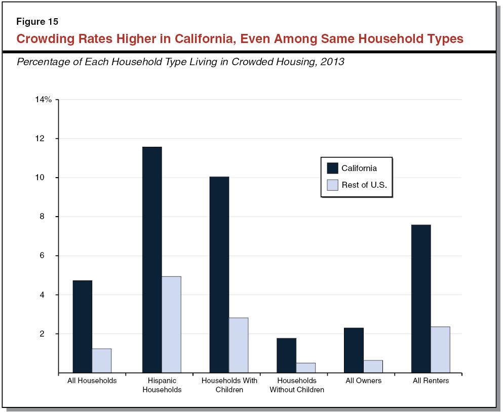
California Households Four Times More Likely to Live in Crowded Housing. Certain household types are more likely than average to live in crowded housing, such as households headed by foreign–born adults, Hispanics, and those with children. California has a higher share of these household types than the rest of the U.S. Because of this, we would expect California to have a higher crowding rate. A review of the data, however, shows that California’s crowding rate is higher than one would expect based solely on its larger share of these household types. This is because crowding rates for each household type (including those most likely to live in crowded housing) are higher in California than they are elsewhere. As a result, California’s overall crowding rate is four times higher than the U.S. average, partly due to demographics and partly to other factors, including higher housing costs, as discussed below.

Crowding Appears Associated With High Housing Costs. Determining whether housing costs affect crowding is challenging because areas with the high housing costs tend to have fewer households types that are likely to be crowded. Using statistical analysis, however, we found that living in a high housing cost area is associated with a higher likelihood of living in crowded housing, after accounting for other factors that also affect crowding rates. Figure 16 shows that the likelihood of being crowded increases when the area’s median home price increases (moving from left to right). For example, the average household’s likelihood of being crowded in a metro with average home prices (about $440,000) is about 3 percent, but the same household’s likelihood of being crowded increases more than threefold—to 10 percent—if they live in an expensive metro with median home prices of $900,000.

Households Commute Further to Work

Each Household Makes Its Own Decisions About Commuting. Housing’s geographic location has lasting and important consequences. Ideally, each household could choose housing in their preferred neighborhood, near good schools and welcoming amenities, with only a short work commute. In practice, though, not only are ideal locations relatively sparse, those that do exist are desirable and therefore expensive. In response, households balance their preferences and resources, selecting trade–offs among housing costs, commute times, and neighborhood characteristics.

Complex Metro Characteristics Influence Commute Times. Each major metro area in the country has unique characteristics that influence whether it has above– or below–average commute times. Most factors are straightforward—for instance, natural geography, existing transportation infrastructure and the availability of public transit, and the spatial distribution of jobs relative to that of housing. Other factors are less straightforward. A metro’s land area and its density affect commute times, but in complex ways. For example, up to a point, commute times generally increase as areas become denser because transportation options become more congested. After densities reach a certain level, however, the viability of public transportation options improves. In some circumstances, this can relieve pressure on other transportation options and reduce average commute times.

California’s Coastal Metros Have Long Commutes. In 2013, workers in large metros throughout the country spent, on average, 55 minutes commuting each day. Workers in California’s coastal metros averaged 60 minutes, about 10 percent more than the national average. Commute times in Los Angeles, the state’s largest metro, averaged 62 minutes, 12 percent longer than the U.S. average. San Francisco has the state’s longest average commutes—72 minutes per day—about 30 percent longer than the U.S. average.

How Might Housing Costs Affect Commute Times? The relationship between metropolitan characteristics, including its housing costs, and average commute times is complex. Assuming neighborhood characteristics and other preferences are unchanged, housing costs should decline as one moves further from job centers. This is because commuting involves monetary and nonmonetary costs that must be offset somehow. Neighborhood characteristics and preferences change across metropolitan areas, however, making the analysis of commute times and metro characteristics additionally complex. To find housing at a price they are willing to pay, households in more expensive metros might choose to live further from work than they would if housing were less expensive. This could lead average commute times to be longer in areas with higher housing costs. Not surprisingly, we found that metro areas with higher housing costs tend to have longer average commute times.

Do High Housing Costs Lead to Longer Commutes? Our analysis found that many important factors have statistically significant effects on commute times. These include: whether the commuter drives, walks, or takes public transit to work; the metro’s land size, population, and density; the metro’s median income; and weather. After controlling for these factors—in essence isolating the effect of housing costs on commute times—a 10 percent increase in a metro’s median rent is associated with a 4.5 percent increase in individual commute times. The fact that California’s average commute times are only moderately above average (despite notably higher housing costs) suggest that other California–specific factors reduce average commute times. These factors may include weather conditions, widespread development and availability of freeway systems, and an above–average share of commuters who drive to work. (Driving commutes are generally fast, and therefore metros with higher shares of driving commuters tend to have shorter commute times.) Despite these mitigating factors, however, our analysis suggests that California’s high housing costs cause workers to live further from where they work, likely because reasonably priced housing options are unavailable in locations nearer to where they work.

Housing Costs Influence Where Households Live and Work

Decisions About Where to Live and Work Are Complex. Understanding how housing costs affect a household’s decision about where to live and work is challenging. This is because regional and state economies are complex and numerous interconnected factors influence housing costs (as well as other costs of living) and economic opportunities in these areas. Despite this complexity, economists and other researchers have identified ways that housing costs affect migration—and, in some instances, have attempted to quantify the magnitude of these effects. Below, we summarize the aspects of this work we believe are most helpful when considering how housing costs affect migration and the state’s economy.

High Housing Costs Discourage People From Living in California. Housing costs are a significant driver of migration to and from California, and changes in the state’s housing costs (relative to other areas of the country) influence migration trends. The ratio of in–migration to out–migration, a measure of population flow, is lowest when California’s home prices are high relative to other places. On the other hand, this flow is highest when California housing becomes relatively more affordable compared to other states. Our analysis of these trends, which we discussed in the preceding section, suggests that about 7 million additional people would live in California if more housing had been built here and the state’s housing prices had therefore grown about as quickly as those in the rest of the country since 1980.

High Housing Costs May Make it Difficult to Recruit Employees. For most businesses, labor costs are their largest operating cost. In areas with higher costs of living, businesses generally must pay employees higher wages because they require additional income to offset the cost of living differences. California’s cost of living is among the highest in the nation, largely because California’s housing costs are so high. As a result, businesses in California’s coastal metros may find it challenging (and expensive) to recruit or retain qualified employees. In a 2014 survey of more than 200 business executives conducted by the Silicon Valley Leadership Group, 72 percent of them cited “housing costs for employees” as the most important challenge facing Silicon Valley businesses. Employee recruitment and retention, closely related to housing costs, was the second most frequently identified challenge. Similarly, other important sectors of the state’s economy may find recruitment challenging and labor costs expensive. For example, some higher education institutions in high housing cost areas provide housing subsidies in order to recruit successfully top administrators and academic specialists. Stanford University recently announced plans to lease a 167–unit apartment complex for their staff and faculty, noting that providing housing helps them “compete to recruit the best faculty from other parts of the country, where they experience very different real estate markets.”

High Housing Costs Mean Fewer Californians Work in State’s Most Productive Cities. In general, businesses and employees in large cities are more economically productive than those in other areas. (Economists use the term “agglomeration economies” to describe these areas. Agglomeration economies are areas where worker productivity increases as population density increases.) Higher productivity leads to more economic output per employee, and thus greater economic growth in the region. Under normal circumstances, these economic opportunities attract new workers from other areas. Historically, this has led to significant population growth in the state’s cities. However, in recent decades, high housing costs have slowed this trend. This is because the expected wage gains (from moving to a city) are not large enough for many prospective workers to make up for their higher housing costs. California’s major productive cities have therefore grown less quickly than they otherwise would.

Fewer Workers in State’s Most Productive Cities Hinders Economic Growth. The slowing flow of workers to productive cities likely has constrained economic growth because potential workers, unable to move to productive cities due to high housing costs, do not benefit from the productivity gains occurring in cities. If more workers lived in the state’s highly productive cities (and therefore reaped these cities’ productivity benefits), per capita economic activity in the state would be greater than it is today. Estimating the magnitude of this impact involves considerable uncertainty. Recent research, however, may provide a helpful guide as to this impact’s order of magnitude. Economists at the University of California, Berkeley and the University of Chicago recently estimated that annual U.S. economic output—the total value of goods and services produced each year—is 13 percent lower today than it otherwise would be due to “increased constraints to housing supply in highly productive cities.”

Looking Ahead: What Is Needed to Contain California’s High Housing Costs?

California’s high housing costs present many difficult issues for policy makers, residents, and businesses to consider. On the one hand, California’s constraints on housing supply—the primary factor driving the state’s high housing costs—show no signs of abating. If California continues on its current path, the state’s housing costs will remain high and likely will continue to grow faster than the nation’s. This, in turn, will place substantial burdens on Californians—requiring them to spend more on housing, take on more debt, commute further to work, and live in crowded conditions. Growing housing costs also will place a drag on the state’s economy.

On the other hand, addressing California’s constraints on housing supply would be extremely challenging and involve major trade–offs. Though the exact number of new housing units California needs to build is uncertain, the general magnitude is enormous. On top of the 100,000 to 140,000 housing units California is currently expected to build, our analysis suggests that the state probably would have to build as many as 100,000 additional units annually—almost exclusively in its coastal communities—to seriously mitigate the state’s problems with housing affordability. Adding this many new homes, however, could place strains on the state’s infrastructure and natural resources and could alter the longstanding and prized character of California’s coastal communities. Facilitating this housing construction also would require the state to make changes to a broad range of policies that affect housing supply directly or indirectly—including many policies that have been fundamental tenets of California government for many years.

Despite these challenges, California’s housing problems warrant attention from state leaders. These difficult issues could require years of legislative deliberation, including discussions with all major stakeholders: the administration, local governments, environmental groups, affordable housing developers and advocates, and housing policy experts. In its deliberations, we recommend that the Legislature:

• Aim to Build More Housing in Coastal Cities, Densely. The greatest need for additional housing is in California’s coastal urban areas. We therefore recommend the Legislature focus on what changes are necessary to promote additional housing construction in these areas.
• Put All Policy Options on the Table. Given the magnitude of the problem, the Legislature would need to take a comprehensive approach that addresses the problem from multiple angles and reexamines major policies. Major changes to local government land use authority, local finance, CEQA, and other major polices would be necessary to address California’s high housing costs.
• Recognize Targeted Role of Affordable Housing Programs. These programs play an important role in assuring housing access for many Californians with unmet housing needs. We note, however, that the scale of these programs—even if greatly increased—could not meet the magnitude of new housing required that we identify in this report. Accordingly, we recommend the Legislature consider how targeted programs could supplement more private housing construction by assisting those with limited access to market rate housing, such as people experiencing homelessness, those with mental and/or physical health challenges, and those with very low incomes.
• Understand That Some Factors Are Beyond Policy Makers’ Control. Much can be done by state and local governments to promote additional housing construction and therefore slow down growth in home prices and rents going forward. Some factors, however, such as high demand to live in the state and natural limitations on developable land, largely are beyond the control of policy makers. As a result, home prices and rents in California likely will remain above–average for the foreseeable future, even if public policies highly favorable to new housing construction were instituted that slowed future growth in housing costs.