LAO Contact

March 7, 2018
Building Reserves to Prepare for a Recession
- Introduction
- How a Recession Leads to a Budget Problem
- State Budget Reserves
- The Governor’s Reserve Proposal
- Planning for a Recession
- Setting a Reserve Target
- LAO Comments
Executive Summary
The Role of Reserves in Preparing for a Recession. Reserves are of critical importance to the health of the state’s budget. In the face of the next recession, these funds will help cushion the impact of the budget problem that emerges. Consequently, setting the level of reserves is one of the Legislature’s most important decisions as it crafts the annual state budget. There is no such thing as an objectively “right” level of budget reserves, so this report provides a framework, with a set of factors, that the Legislature can use to determine its target.
Recessions and Budget Problems
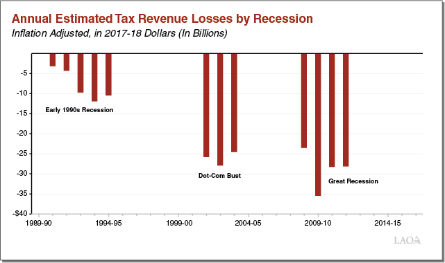
Revenue Losses. California’s tax structure is quite volatile. Revenues fluctuate in response to underlying changes in the economy and stock market more than most other states. The figure below shows revenue losses over the past three recessions—which have totaled in the tens of billions of dollars over multiyear periods. The Great Recession was the most severe. However, even the dot‑com bust in the early 2000s, which in economic terms was more moderate, led to over $80 billion in losses.
Budget Problem. A budget problem represents the amount by which expenditures exceed revenues in a given year. A budget problem is not the same as a revenue loss. That is because some state expenditures adjust automatically to changing revenue conditions, in general offsetting losses. We estimate that, on average, automatic adjustments offset roughly half of an initial revenue loss. To put this in more concrete but very rough terms, a moderate recession, like the dot‑com bust, could lead to a $40 billion budget problem. A more mild recession might result in a $20 billion budget problem.
Planning for a Recession
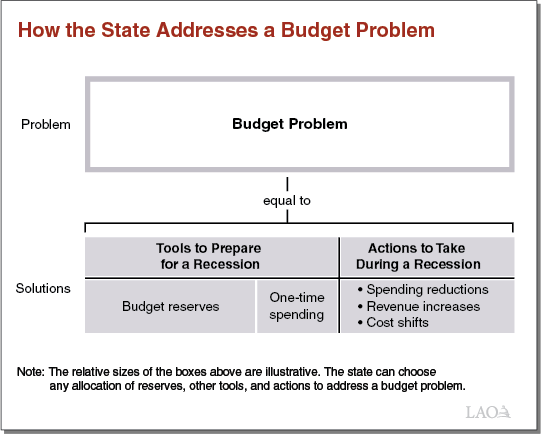
Framework to Plan for a Recession. In this report, we present a framework to help the Legislature plan for the next recession. First, we suggest the Legislature consider the size of the recession for which it would like to prepare. Second, we suggest the Legislature consider how it would like to respond. As shown in the figure below, there are basically two means: (1) tools that allow the state to prepare in advance of a recession and (2) actions the state must take during a recession. In particular, in preparation for a recession, the state can build budget reserves and spend money on a one‑time basis. These actions reduce the size of a potential budget problem later. During a recession, if a budget problem persists, the state must take actions to address it. These actions include spending cuts, revenue increases, and cost shifts. Together, the sum of all these responses equals the size of the budget problem.
Reserves This Year
Governor Proposes Nearly $16 Billion in Reserves. In his 2018‑19 budget plan, the Governor proposes the state enact a reserve level of $15.7 billion, the highest in recent decades. The Governor executes this proposal by making an optional $3.5 billion deposit into the state’s rainy day fund, bringing it to its constitutional maximum. While the Governor’s proposed level would be historic for California, it is not particularly remarkable by national standards.
Is the State Adequately Prepared for the Next Recession? For context, this level of reserves would allow the state to weather a mild recession with nearly no additional actions. However, if the state faced a moderate recession with this level of reserves, it would also have to take roughly $25 billion in actions to address a budget problem, including spending cuts, revenue increases, and cost shifts. The Governor’s reserve proposal, therefore, raises fundamental questions about the state’s current—and potential future—level of reserves. In particular: Is the Legislature satisfied with this level of preparation for the next recession?
Governor’s Proposal, Counterintuitively, Makes Building More Reserves More Difficult. Given all of the uncertainties that the budget currently faces, we think the Governor’s proposed level of reserves is a reasonable minimum. However, the specifics of the Governor’s reserve proposal—counterintuitively—make building more reserves in the future more difficult. That is because reaching the rainy day fund’s maximum level means that funds which would have been deposited into reserves must instead be spent on infrastructure. This lowers the amount of resources available for building more reserves in the future by roughly $1 billion per year.
Alternatives to Build More Reserves. As such, if the Legislature’s target level of reserves for this year, or a future year, is greater than $16 billion, it might consider using another more effective way to build reserves. In this report, we offer some alternatives for consideration that would help the Legislature build more reserves than the Governor is currently proposing. These include options outside of the rainy day fund, as well as other budgetary tools that have the same key attributes of reserves. Relative to what the Governor now proposes, using one of these alternatives would help make the state even better prepared for a coming recession.
Introduction
In his 2018‑19 budget plan, the Governor proposes a total reserve balance of nearly $16 billion, including a discretionary deposit of $3.5 billion into the state’s rainy day fund. This proposed deposit would fill the reserve to its constitutional maximum level. This action raises an important question for the Legislature to now consider: Does the currently proposed level of reserves sufficiently prepare the state for the next recession?
Setting the budget’s level of reserves is one of the Legislature’s most important decisions as it crafts the annual state budget. As there is no such thing as an objectively “right” level of budget reserves, the Legislature’s target each year can depend on a variety of factors. In this report, we present a framework for the Legislature to use to determine its target level of reserves using a set of specific and measurable factors.
This report first describes how a recession leads to a budget problem—the primary reason the state holds budget reserves. Next, it describes California’s policies and practices on reserves. Then, the report presents the Governor’s reserve proposal for the 2018‑19 budget and considers the proposed level both historically and among other states nationally. Next, to aid the Legislature as it evaluates the Governor’s proposal, the report presents a framework that the Legislature can use to plan for a recession and determine a target level of reserves. Finally, we conclude with our office’s comments on the Governor’s proposed level of reserves in light of this framework and present some alternatives for legislative consideration.
How a Recession Leads to a Budget Problem
Budget reserves help cushion the impact of budget problems—that is, when revenues are insufficient to cover expenditures. The primary reason the state would face such a shortfall is due to an economic recession. (As described in the nearby box, the state also can use budget reserves to cover the cost of large unanticipated, one‑time expenses.) In this section, we describe how a recession leads to a budget problem. First, we describe how recessions affect state revenues, quantifying the revenue losses that have occurred in recent downturns. Then, we describe how recessions tend to affect state expenditures. The net of these two factors is the size of the state’s “budget problem.”
Reserves Can Be Used for One‑Time, Unanticipated Expenses
One‑Time, Unanticipated Expenses. In addition to recessions, the budget sometimes relies on budget reserves to cover the cost of significant, but one‑time, unanticipated expenses. The most sizeable of these are often related to natural disasters and other crises. Compared to budget shortfalls that occur as a result of revenue declines during an economic recession (which result in losses of tens of billions of dollars over multiyear periods), these budgetary costs are relatively small.
Examples of Significant Past Costs. The state has incurred notable one‑time expenses as a result of several major events. (The state often receives significant reimbursements from the federal government for the cost of natural disasters, but federal aid does not cover the entire cost.) Most recently, state costs of the 2017 California wildfires, while still evolving, are currently projected to be in the high hundreds of millions of dollars. Other examples of significant past events include:
- Energy Crisis. When the state’s two largest utilities faced serious financial problems in the early 2000s, the state Department of Water Resources began purchasing electricity on behalf of the utilities’ customers. The state used proceeds from the sale of long‑term electricity bonds to finance $11.2 billion in these costs. (Electricity ratepayers, rather than General Fund taxpayers, repaid these bonds financed by a surcharge on electricity bills.) In addition, in response to the crisis, the state spent $1 billion (roughly $1.5 billion in today’s dollars) on various conservation and rebate programs in the 2001‑02 budget.
- Loma Prieta Earthquake. In 1989, an earthquake in Northern California resulted in severe damage to infrastructure in cities across the region, including the partial collapse of the San Francisco‑Oakland Bay Bridge. In response to the earthquake, the state increased the sales tax by a quarter cent to raise $800 million ($1.6 billion in today’s dollars) for disaster relief.
- Paterno Lawsuit. In a 2003 decision in Paterno v. California, a state appellate court found the state was responsible for a levee failure along the Yuba River in 1986. The state eventually paid a $464 million settlement to the nearly 3,000 plaintiffs.
- January 1997 Floods. Major flooding in Central and Northern California occurred at the very beginning of 1997 after a week of heavy rainfall. The floods resulted in disaster declarations in 48 counties and forced more than 120,000 from their homes. After federal reimbursements, these floods led to nearly $200 million in state costs (over $300 million in today’s dollars).
Recessions and Revenue Declines
Recessions are technically defined as six months of decline in a country’s gross domestic product (GDP), a broad measure of the size of an economy. Recessions are often characterized by rising unemployment rates and losses in asset markets (for example, stocks and real estate). Below, we describe how recessions affect state revenues, with a focus on revenue losses that have occurred in recent recessions.
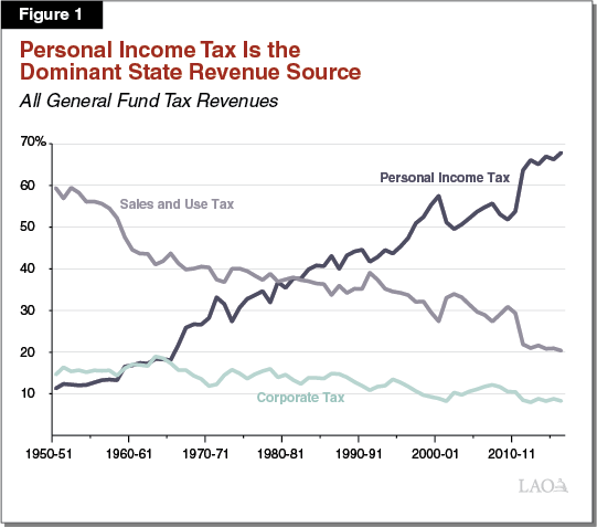
Personal Income Tax Is Dominant State Revenue Source. The personal income tax (PIT) is the state’s tax on most sources of individual income, including: salaries and wages, proprietor and partnership income, capital gains, dividends and interest, and retirement distributions. As Figure 1 shows, the PIT makes up almost 70 percent of state General Fund revenues. The sales and use tax (SUT)—which is levied on most tangible personal property sold and used in California—is the second largest General Fund revenue source. The corporation tax, which is levied on corporate income, is the third. Although all three of the largest General Fund revenue sources have grown over time, the SUT has declined significantly as a share of overall General Fund revenues. This decline has occurred in large part because the prices of services (such as health care), which are not subject to the sales tax, have grown faster than the prices of goods.
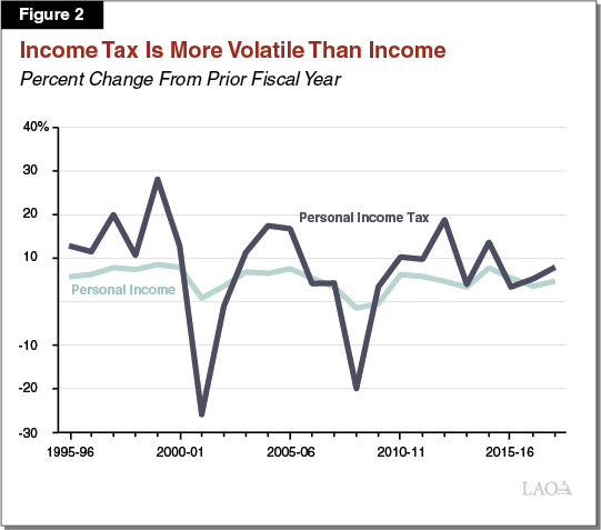
PIT Experiences Large Losses During Downturns, Increases During Expansions. Personal income grows each year when the economy is expanding and either shrinks or grows more slowly when the economy is not growing. As a result, the growth rate of PIT revenue fluctuates from year to year. Figure 2 shows that revenues associated with the PIT experience more significant year‑over‑year changes than personal income itself. There are a variety of reasons for this. These include: (1) the inclusion of capital gains into the PIT base (although they are not included in the definition of personal income) and (2) the PIT’s progressive rate structure.
Revenue Losses Associated With Past Recessions. Figure 3 shows estimates of tax revenue losses associated with each of the last three recessions: the recession of the early 1990s, the dot‑com bust and ensuing recession in the early 2000s, and the financial crisis and Great Recession beginning in 2008. These estimates are calculated by comparing actual revenues (after adjusting for major revenue changes) to a baseline case where revenues continued to grow at their historic rate. (We would note, however, that this exercise is not precise and different measures of revenue losses could be higher or lower by billions of dollars.) We estimate that revenue losses, in inflation‑adjusted terms, totaled roughly $40 billion in the 1990s (averaging $8 billion per year across five years), $80 billion in the early 2000s ($26 billion per year across three years), and about $115 billion during and after the Great Recession ($30 billion per year across four years). As the figure suggests, the state does not need to endure severe economic problems to experience significant revenue losses.
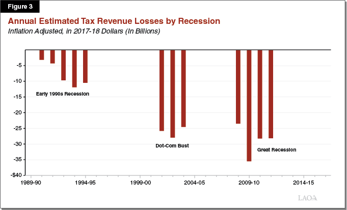
Size of the Recession Does Not Perfectly Predict Revenue Losses. In general, larger recessions result in more revenue losses, but the relationship is not perfect. By most measures, the recession of the early 1990s was more severe than the dot‑com bust in the early 2000s. For example, unemployment in California reached 9.7 percent in mid‑ to late‑1992, but peaked at 6.9 percent after the dot‑com bust. However, as noted earlier, revenue losses in the early 1990s were much smaller than those in the early 2000s. Two major factors help to explain this. First, between 1990 and 2000, the General Fund became increasingly reliant on PIT revenues, relative to SUT revenues, which are much less responsive to economic conditions. As a result, revenue volatility increased between these two events. Second, the dot‑com bust involved much more significant losses in the stock market, which affect capital gains revenues.
General Fund Revenue Volatility Has Likely Increased Since Last Recession. Since the Great Recession ended, changes in the state’s policies and economy have likely increased the volatility of General Fund revenue. Proposition 30 (2012) enacted, and Proposition 55 (2016) extended, tax increases on high‑income taxpayers whose income is especially sensitive to fluctuations in the economy and asset markets. In addition, the 2011 realignment of state and local government responsibilities reduced General Fund revenue from the sales tax, a more stable revenue source. As a result of both of these policy changes, the structure of General Fund revenue is likely more sensitive to shifts in the economy and asset markets than it was in the past. In addition, income growth in recent years has been especially fast at the higher end of the state’s income spectrum, which creates more volatility in the PIT base. Together, these changes to the PIT structure and base likely mean that similarly sized recessions in the future could lead to larger General Fund revenue losses.
Recessions and Spending Changes
While the Legislature makes programmatic adjustments in response to changing budgetary conditions, some spending levels change “automatically,” either as a result of formulas, caseload, or price changes. Some programs tend to expand in a recession, while others tend to decline.
Proposition 98 Spending Generally Declines During a Recession. Proposition 98 (1988) governs most state funding for schools and community colleges. The measure establishes formulas for a minimum annual funding requirement, commonly referred to as the minimum guarantee. The minimum guarantee rises or falls with a variety of inputs, including: General Fund revenue, per capita personal income, and K‑12 student attendance, among other factors. The formulas also provide for “maintenance factor,” which requires the state to accelerate school funding in strong revenue years to compensate for lower funding in weaker years. Given these formulas, General Fund spending on schools and community colleges tends to increase when revenues are growing and decline when revenues decline. The Legislature can provide more than the minimum funding level for schools and community colleges, but it typically funds at the guarantee.
Proposition 2 Requirements Also Decline During a Recession. Proposition 2 (2014) requires the state to make minimum annual reserve deposits and payments toward certain eligible debts. Discussed more later in this report, under the provisions of Proposition 2, the state makes these deposits and payments based in large part on the performance of General Fund revenues, particularly those from capital gains. When revenues are higher, these requirements are higher and vice versa. This means that Proposition 2 offsets revenue losses, in some part, during a recession, by automatically declining.
Caseload‑Driven Spending Generally Increases During a Recession. The funding levels for some programs, particularly in health and human services, depend on a combination of changes in their number of participants (caseload), the costs per enrollee (price), and the intensity at which participants use services (utilization). Examples of these programs include Medi‑Cal (the state’s Medicaid program) and CalWORKs, which provides cash assistance and services to low‑income individuals. During a recession, these programs’ caseloads (and hence their costs) tend to rise as more people become eligible for their services.
The Budget Problem
A budget problem represents the amount by which expenditures exceed revenues in a given year. A budget problem is not the same as the revenue loss the state experiences during a recession. That is because, as described in the previous section, some state expenditures adjust automatically to changing revenue conditions. In particular, increases in spending contribute to a larger budget problem and declines reduce the size of the budget problem. The budget problem faced by the state is the net effect of changes in both revenues and expenditures.
Formula‑Driven Reductions Can Offset Roughly Half of Revenue Losses. Over the last few years, our annual Fiscal Outlook publications have shown a hypothetical budget problem that would arise from varying levels of revenue losses for the state. Under different scenarios ranging from a slowdown in growth to a moderate recession, estimated revenue losses have ranged from $30 billion to $80 billion over a multiyear period. In each of these scenarios, automatic adjustments to spending have offset roughly half of the revenue loss.
State Budget Reserves
How Reserves Insulate the Budget. Budget reserves are monies set aside for future use, like a household’s savings account that is dedicated to emergencies. Reserves help insulate the budget from temporary shortfalls, delaying or mitigating the need for the Legislature to make difficult choices, including spending reductions and tax increases.
State Has Two Budget Reserves. The state has two budget reserves: the Special Fund for Economic Uncertainties (SFEU) and the Budget Stabilization Account (BSA). The SFEU is the state’s discretionary budget reserve—that is, the Legislature at any time can appropriate SFEU funds for any purpose by majority vote. Use of funds in the state’s rainy day fund—the BSA—is more restricted. The State Constitution has specific rules regarding how and when the state must make deposits into, or may make withdrawals from, the BSA. Below, we describe the major policies that guide these two budget reserves.
Special Fund for Economic Uncertainties
SFEU Is the State’s Discretionary Reserve. The 1980‑81 Budget Act established within the General Fund the Reserve for Economic Uncertainties. In 1985, the fund was renamed the Special Fund for Economic Uncertainties. Simply put, the SFEU is the difference between spending and available resources (most notably, revenues) for a given fiscal year. In any year, its balance (the amount by which resources available exceed spending) is the state’s discretionary reserve.
Enacted SFEU Balance Cannot Be Less Than Zero. The California Constitution requires the state to enact a balanced budget each year. Specifically, Article IV prohibits the Legislature from enacting a budget bill that would appropriate more in General Fund expenditures than are available in resources. In effect, this means the estimated balance of the SFEU—at the time of the budget’s passage—cannot be lower than zero. However, budget estimates rely on projections of future revenue that are inevitably uncertain. As such, a deficit can emerge in the SFEU after the passage of the budget, which can be carried into the next fiscal year.
Large SFEU Balance Triggers Tax Reductions. California has two statutes that trigger reductions in the state’s sales tax rate if balances in the SFEU reach a certain threshold. Under either statute, the state’s sales tax rate would automatically decline by one‑quarter cent for one calendar year, equal to around $1.7 billion, reducing the SFEU by the same amount. Under the first statute, the trigger would occur if the Director of Finance projects the SFEU to exceed about 4 percent of General Fund revenues (currently, about $5.4 billion) in the prior and current year. Under the second statute, the trigger would occur if (1) the “General Fund reserve” exceeds about 3 percent of revenues (currently, around $4 billion) and (2) actual General Fund revenues between May 1st and September 30th exceed the administration’s forecasted amounts.
Budget Stabilization Account
Proposition 58 Governed BSA From 2004 to 2014. Until 2014, the BSA was governed by Proposition 58. Passed by voters in 2004, Proposition 58 required the state to make an annual transfer into the BSA. These required deposits were to gradually increase from 1 percent of General Fund revenues in 2006‑07 to 3 percent in 2008‑09 and every year thereafter. Proposition 58 allowed these deposits to be suspended by an executive order issued by the Governor. Between 2004 and 2014 only two transfers were made to the BSA under the provisions of Proposition 58. These deposits were made in the 2006‑07 and 2007‑08 enacted budgets when the economy was still expanding, but were quickly used to address budget deficits that emerged later on in the 2007‑08 fiscal year. Before 2004, Proposition 98 required the Legislature to maintain a “prudent state reserve fund” in the amount deemed “reasonable and necessary.”
Proposition 2 Changed BSA Rules. In 2014, voters passed Proposition 2, amending the rules concerning deposits into and withdrawals from the BSA. Under the measure, the amount of each annual deposit is determined as follows:
- First, the state must set aside 1.5 percent of General Fund revenues (we refer to this as the “base amount”).
- Second, the state must set aside a portion of capital gains revenues that exceed a specified threshold (we refer to this as “excess capital gains”).
The state combines these two amounts and then allocates half of the total to pay down eligible debts and the other half to increase the balance of the BSA.
Legislature Has Limited Control Over BSA Deposits and Withdrawals. Under the rules of Proposition 2, the Legislature can only reduce the BSA deposit, or make a withdrawal from the BSA reserve, in the case of a budget emergency. This can only occur upon declaration by the Governor and majority votes of both houses of the Legislature. The Governor may call a budget emergency in two cases: (1) if estimated resources in the current or upcoming fiscal year are insufficient to keep spending at the level of the highest of the prior three budgets, adjusted for inflation and population (a “fiscal budget emergency”) or (2) in response to a natural or man‑made disaster. In the case of a fiscal budget emergency, the Legislature may only withdraw the lesser of: (1) the amount needed to maintain General Fund spending at the highest level of the past three enacted budget acts, or (2) 50 percent of the BSA balance.
Constitution Requires “True Up” of BSA Deposits. Under Proposition 2’s true‑up provisions, the state reevaluates each year’s BSA deposit twice: once in each of the two subsequent budgets. The state does this because initial estimates of future capital gains revenues are highly uncertain. This process attempts to align those original estimates with actual revenues. Under these reevaluations, the state revises the BSA deposit up or down if excess capital gains taxes are higher or lower than the state’s prior estimates. The state does not revisit its estimate of the base amount or debt payments in the true‑up calculation.
Constitutional Deposits Are Lower Once BSA Reaches Maximum Size. Under Proposition 2, the state must put money into the BSA until its total reaches a maximum amount of 10 percent of General Fund tax revenue. Currently, this is about $13.5 billion. Once the BSA reaches this maximum, funds that would bring the BSA above 10 percent of General Fund taxes must be spent on infrastructure. Each year that General Fund tax revenues grow, the maximum level of the BSA also grows. So each year that the state does not face a fiscal budget emergency, it would continue to make deposits into the BSA to bring the fund to the revised estimate of 10 percent of General Fund taxes. These deposits would be hundreds of millions of dollars per year, with the remainder going toward infrastructure spending.
The Governor’s Reserve Proposal
This section summarizes the Governor’s reserve proposal in the 2018‑19 budget and places the proposal in context—both historically and nationally.
Governor Proposes $15.7 Billion in Total Reserves. In his 2018‑19 budget plan, the Governor proposes ending the year with $15.7 billion in total reserves (see Figure 4). This would consist of two amounts: $13.5 billion in the BSA and $2.3 billion in the SFEU. The administration currently estimates a very small “true down” to the BSA in 2017‑18, although that may change at the time of the May Revision. (We believe there is significant upside to the administration’s 2017‑18 revenue estimates, which would result in a required true up deposit.)
Figure 4
Total Reserves Proposed in the Governor’s 2018‑19 Budget
(In Billions)
|
Special Fund for Economic Uncertainties (SFEU) |
|
|
Enacted SFEU in 2017‑18 budget |
$1.4 |
|
Additional SFEU balance proposed in 2018‑19 |
0.9 |
|
Subtotal |
($2.3) |
|
Budget Stabilization Account (BSA) |
|
|
Balance enacted in 2017‑18 budget |
$8.5 |
|
True up deposit for 2017‑18a |
‑0.1 |
|
Required 2018‑19 deposit |
1.5 |
|
Optional 2018‑19 deposit (proposed) |
3.5 |
|
Subtotal |
($13.5) |
|
Total |
$15.7 |
|
aThe administration currently estimates a small “true down” deposit for 2017‑18, which would reduce the BSA’s balance by $75 million. |
|
Governor Proposes Reaching BSA Maximum With Optional Deposit. The Governor proposes making an optional deposit into the BSA that would bring the account to its constitutional maximum (10 percent of General Fund taxes or, currently, $13.5 billion). Under the administration’s current proposal and revenue estimates, the additional deposit needed to reach the BSA’s constitutional maximum is $3.5 billion. In May, if the administration does increase its revenue estimates for 2017‑18 and estimates a true up deposit is required, it is likely to reduce the optional deposit by the same amount, keeping the overall proposed BSA balance the same.
Governor Proposes Making Optional Deposit Statutorily Subject to BSA Rules. The Governor proposes statutory language that would aim to limit the Legislature’s access to the optional BSA deposit under the traditional rules governing constitutional deposits. (This statutory language could be amended in the future.) Under the Governor’s proposal, the Legislature could only access those funds if specific budget emergency conditions exist and the Governor calls a budget emergency. Moreover, even in the case of a budget emergency, the amount of a withdrawal could not exceed 50 percent of the BSA balance in the first year. (The Governor proposed, and the Legislature approved, an optional BSA deposit of $2 billion in the 2016‑17 budget, which was executed using similar statutory language.)
Governor’s Proposal Creates Infrastructure Spending Obligation in 2019‑20 and After. If the Legislature approves the Governor’s proposal to reach the BSA maximum, a portion of future years’ Proposition 2 requirements must be expended on infrastructure. Under the administration’s current projections, this would result in a $959 million infrastructure spending requirement in 2019‑20, $947 million in 2020‑21, and $987 million in 2021‑22. These are funds that—absent the proposal—would have been deposited into the BSA under the administration’s own multiyear projections.
Proposed Reserves in Context
This section compares the Governor’s proposed level of reserves to California’s historical averages and then to other states.
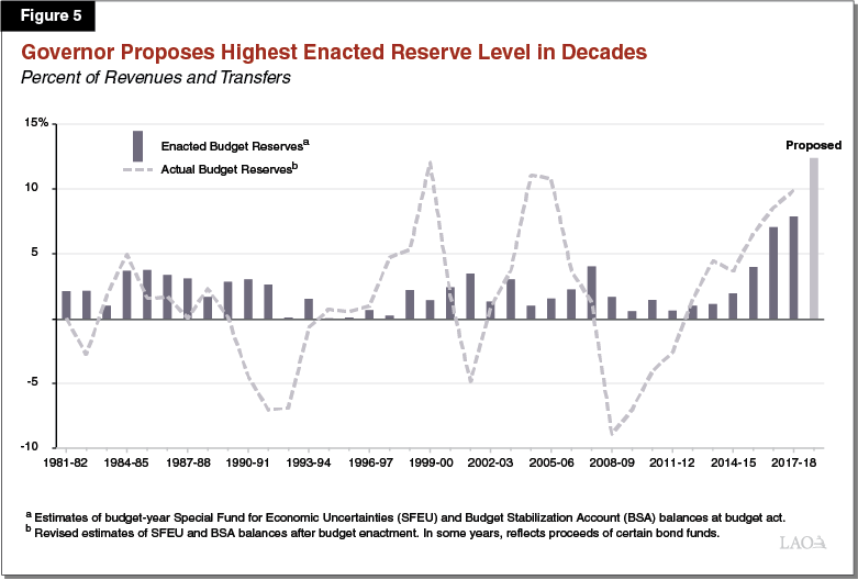
Governor Proposes Highest Enacted Reserve Level in Decades. Figure 5 compares the Governor’s proposed level of reserves to a history of California’s enacted and actual budget reserves. The blue bars display enacted reserves, or the amount of combined SFEU and BSA reserves that was assumed in the annual state budget for the upcoming fiscal year at the time it was enacted. The dashed line shows actual reserves, or the revised level of reserves estimated by the Department of Finance for prior years, after the state has more information about realized revenues and expenditures. As the blue bars in the figure show, over the last few years, California has been enacting reserve levels above 5 percent—well above averages in the last few decades. If the Governor’s proposed level of reserves is enacted, it would represent the highest level of enacted reserves held by the state in decades. As discussed earlier, the balanced budget provisions of the State Constitution require the state to enact a positive SFEU balance, but actual reserves fluctuate around zero.
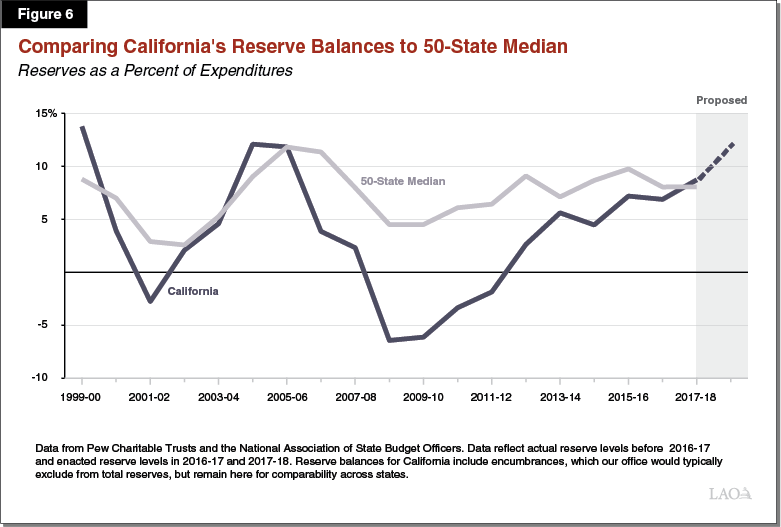
Other States Are Maintaining Similar Reserve Balances. While unusual for California, the state’s recent reserve balances are only slightly higher than the median reserve level across all 50 states. Figure 6 compares median reserve balances across all states to California over 20 years. The chart shows enacted reserves for 2017‑18, updated reserve estimates for 2016‑17, and actual reserve estimates for all previous years. Historically, California’s reserve levels have been much lower than median reserves across all states, particularly during recessions. In 2017‑18, median enacted reserve levels stood just over 8 percent of expenditures, near California’s enacted level. The Governor’s proposed reserve balance of 12 percent is somewhat above that level. (We would note that reserve levels across states are not always directly comparable.)
Revenue Volatility Varies by State. Different states rely on different mixes of taxes and fees for their General Fund revenues. For example, some states rely on general or selective sales taxes as their primary revenue sources, which tend to be more stable revenue sources. Even among states with significant PIT revenues, the structure and composition of those taxes can vary. For example, California has a graduated rate structure and taxes capital gains as regular income. Other states with broad‑based PITs have different features. Some levy these taxes at a flat rate, tax different forms of income, and/or include different credits and deductions. All of these features can play significant roles in revenue volatility.
Comparing Volatility and Reserves. Figure 7 compares a measure of a state’s revenue volatility score, estimated by the Pew Charitable Trusts, to its enacted reserve level in 2017‑18. Pew measured each state’s volatility score by calculating the average variation in the percent change in a state’s revenue (after adjusting for policy changes). As the figure shows, California’s revenue volatility score of 8.5 is well above average and ranks fifth overall. However, California’s enacted level of reserves was near the median level in 2017‑18. Although we might expect states with higher volatility scores to have accumulated higher levels of reserves at this point in the economic cycle, that does not generally appear to be the case.
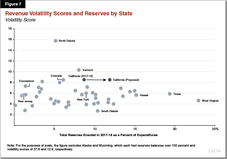
States Reliant on PIT. There are a few other states that, similar to California, rely on the PIT as a major General Fund revenue source and have relatively sizable populations of wealthier people (which tends to make PIT revenues more volatile). These states include Connecticut, Colorado, New York, and New Jersey. As a percent of total expenditures, California’s reserve losses in the Great Recession were greater than all of these states. In recent years, however, reserves in California have caught up to, and then surpassed, balances in these other states. Anecdotally, California appears to be experiencing more growth in its PIT base than these others. For example, Colorado has experienced slower overall growth in General Fund revenues in recent years, driven primarily by slower growth in individual income taxes and losses in corporate income taxes. Connecticut, similarly, has been experiencing slower growth in PIT revenues. Officials in that state say these appear to be related to slower growth overall in the state’s economy. Coupled with cost pressures in major state programs, both of these states have had stagnant growth in reserves.
States Reliant on Severance Tax Revenues. Unlike California, some states levy taxes on the extraction of nonrenewable resources, like oil and natural gas. These “severance taxes” are usually levied on producers as a fixed percent of the commodity’s market value, so the revenue per barrel or other unit of measure varies when the price of the commodity rises and falls. As a result, these revenue sources tend to be very volatile, usually much more so than PIT revenues. Three states in particular—Alaska, North Dakota, and Wyoming—all have a high reliance on severance tax revenue, with 30 percent or more of their overall General Fund revenue coming from this source. These states tend to maintain much higher reserve balances than California. North Dakota’s reserve balance stood at 84 percent of General Fund expenditures in 2010‑11, but has diminished in recent years. Over the past 20 years, Wyoming’s balance has averaged about 44 percent of General Fund expenditures and currently stands over 100 percent.
Proposed Level of Reserves Is Not Remarkable by National Standards. In short, while a historical level for California, total reserves currently proposed by the Governor are only somewhat above average by national standards. The proposed level is higher than the level held by some states with similarly volatile revenue structures, including other PIT reliant states. However, there is little evidence of a strong relationship between states’ revenue volatility and their current level of reserves. Moreover, other PIT reliant states have experienced challenges in revenue collections that California has not seen. So, while it might seem positive that California has built higher reserve levels than these states, given their recent challenges, it could be the case that their reserve levels should be higher—not the other way around.
Planning for a Recession
In this section, we describe a framework that the Legislature can use to plan for the state’s next recession.
Overview of the Framework. To plan for a recession, we suggest the Legislature first consider the size of a recession—and its associated budget problem—for which it intends to prepare. Then, we would suggest the Legislature decide what combination of responses it would like to use to address the budget problem. Figure 8 shows the two available methods. They are:
- Tools to Prepare for a Recession. The Legislature has two main tools to prepare for a recession. They are: (1) budget reserves and (2) one‑time spending.
- Actions to Take During a Recession. If these tools are insufficient to cover the entire shortfall, the Legislature must take actions during a recession to bring the budget into balance. These actions include: (1) spending reductions, (2) revenue increases, and (3) cost shifts.
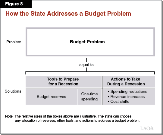
Together, the dollar amount of these two responses must add to the total size of the budget problem. The rest of this section describes each of these factors in turn.
Anticipating the Recession and Budget Problem
In this planning process, we first suggest the Legislature determine the size of a recession—and associated budget problem—for which it would like to be prepared.
Anticipating the Next Recession. No one can predict the timing, size, or length of the next recession. However, the state still must make budgetary decisions in anticipation of such an event. The Legislature’s assessment of the size and timing of the next recession therefore follows from both its assessment of the probability of various events occurring and how cautious it would like to be. As such, when deciding its target level of reserves, the Legislature should first consider the size of the next recession—and associated budget problem—for which it would like to prepare. In general, being prepared for a large recession involves higher levels of reserves.
Rough Illustrations of Possible Budget Problems. From past experience and our understanding of current revenue volatility, we would very roughly estimate that the state would face revenue losses of around $40 billion, with a $20 billion budget problem, in a mild recession. A more moderate recession might involve revenue losses of $80 billion, with a $40 billion budget problem. The Legislature could also choose to prepare for an even larger downturn—for example, one comparable to the Great Recession, although such an event is less likely to be part of the state’s future experience.
Addressing the Budget Problem
After the Legislature has decided the size of the recession and associated budget problem for which it would like to prepare, planning for that recession involves considering two available methods for addressing the budget problem. These are described below.
Tools to Prepare for a Recession
Budget Reserves. As discussed throughout this report, budget reserves are the most important tool the Legislature has to address a budget problem. Making deposits into reserves has two key features that help the budget’s bottom line during a recession. First, making the deposit rather than increasing ongoing spending lowers the spending base, shrinking the size of any future budget problem. Second, making a deposit increases the reserve available later to address a future budget problem.
One‑Time Spending. Another important tool the budget has to prepare for a recession is one‑time spending. One‑time spending has the first benefit of reserves as it does not increase the ongoing expenditure base, thereby reducing the size of a subsequent budget problem. It does not, however, have the second benefit of reserves (setting aside funds for future use). There are two important types of one‑time spending in the budget. They are:
- One‑Time General Fund. Some forms of one‑time General Fund spending more clearly reduce the pressure for ongoing spending than others. For example, appropriating funds for debt payments or information technology projects often does not create an ongoing expectation for future funds for these purposes. One‑time spending on other items—such as new programs, services, or grants—can be more difficult to choose not to repeat.
- One‑Time Proposition 98. The formulas governing Proposition 98 generally provide for a lower minimum guarantee when state revenue is sluggish or declining. Funding at this lower guarantee, however, sometimes requires the state to make difficult choices about reducing funding for core educational programs. One‑time spending within Proposition 98 (for example, per‑student discretionary grants) creates a buffer that allows the state to fund at a lower level during tough economic times with fewer reductions to these core ongoing programs.
Actions to Take During a Recession
If the above tools are insufficient to cover the entire budgetary problem, the Legislature must use a set of actions to address the remaining problem. There are three broad categories of these actions: spending reductions, revenue increases, and cost shifts. We describe some examples of these actions that the Legislature has taken in the past in response to budget problems.
Increase Revenues. To increase revenues, past budgets have, most notably, increased taxes. For example, the 2009‑10 budget temporarily increased the state sales tax by 1 cent and the PIT rates by 0.25 percentage points. Similarly, in 2012, voters passed Proposition 30, which temporarily increased the SUT by one‑quarter cent and increased PIT rates on high‑income earners. The state has also increased fees, suspended tax credits and deductions, increased penalties, and increased resources to enhance taxpayer compliance.
Reduce Spending. The state has taken a variety of actions to reduce spending in past budgets. Some examples include:
- Reducing Services. The state has reduced spending by making both across‑the‑board and targeted cuts by service or program. For example, the state has reduced spending on health and human services programs, corrections, courts, and universities.
- Suspending Mandates. Proposition 4 (1979) requires the state to reimburse local governments for some programs and services the state requires them to provide. In some cases, to achieve budgetary savings, the state suspended these requirements and the associated reimbursements.
- Stopped Providing Cost‑of‑Living Adjustments (COLAs). The budget has historically provided COLAs, or adjustments to programmatic and departmental spending to account for erosions in spending power that result from inflation. During past recessions, the state has not provided COLAs for state employee pay and recipients of health and human services programs, like CalWORKs.
Shift Costs. When facing a budget problem, the state has also taken actions that allowed it to provide services without paying for their full costs at the time. In some cases, these actions have resulted in increased costs to other entities (including local governments). In other cases, these actions shifted costs to future taxpayers by creating a liability that must later be addressed. Some types of actions have since been prohibited by approved ballot measures or were actions that could only be done once. As described in the nearby box, in past recessions the federal government has taken actions that shift costs away from the state, but these are generally outside of the state’s control. In the past, state cost shifts have included:
- Deferrals. Over many years, the state deferred payments to school districts to achieve budget savings. Sometimes this meant making payments a few weeks late—for example, at the beginning of July instead of the end of June. In other cases, however, the state shifted payments by several months. These longer shifts placed a cash burden on school districts, which meant they either had to use their internal reserves or face external borrowing costs. In the past, the state also deferred mandate reimbursements to local governments, which generally shifted state costs onto these entities. Today, Proposition 1A (2004) restricts the state’s ability to defer most mandate reimbursements.
- Internal Loans. To address past budget shortfalls, the state has also made loans to the General Fund from other state accounts known as special funds, generating one‑time savings equal to the loans. The General Fund is required to repay special funds when needed to ensure the special fund meets the object for which it was created. The state has been repaying these outstanding amounts as part of Proposition 2 debt payment requirements over the last few years.
- External Loans. In 2004, voters passed Proposition 57, which authorized the state to issue a bond of up to $15 billion to address its budget shortfall. Proposition 58, passed in conjunction with Proposition 57, prohibits this practice in the future.
- Other Actions. Past budgets have taken a variety of other actions to achieve savings. The 2003‑04 budget shifted the Medi‑Cal program from an accrual basis (where expenditures are booked to the year the obligation is generated) to a cash basis (where expenditures are booked to the year the payments are made). This resulted in one‑time savings of $930 million. Such actions can only be done once unless they are later undone. During the Great Recession, the state also attained budget savings by furloughing state employees.
Changes in Federal Policy That Shift Costs Away From State
In past recessions, the federal government has taken actions to ease states’ budgetary situations. In some cases, increased federal funds can backfill some General Fund spending declines. For example, the American Recovery and Reinvestment Act (ARRA), passed by Congress in February of 2009, provided temporary and one‑time funds to California to backfill some state spending. In particular, the 2009‑10 budget package included an estimated $8.5 billion in federal funds from ARRA to offset General Fund spending. In other cases, the federal government has provided the state with more flexibility to reduce state‑funded programs that it regulates. These changes, however, are often outside of the state’s control in the budget process and therefore are not considered as part of the framework in this section.
Some Spending Solutions Shift Costs. This framework discusses spending and revenue changes separately from cost shifts. However, in many cases, spending reductions result in cost shifts. For example, in past recessions, the state has reduced General Fund spending on the University of California and Califoria State University. To maintain student services, the two university systems have responded by raising fees and tuition, shifting costs to students and their parents.
Setting a Reserve Target
This section discusses how the Legislature can determine its target level of budget reserves using some illustrative reserve targets that provide more specific examples of the framework discussed.
How to Set a Reserve Target. Setting the state’s reserve target is one of the most important decisions for the Legislature as it crafts each year’s budget. A target level of reserves is determined in conjunction with all of the other factors discussed in the previous section. Figure 9 shows how this could work in practice in a variety of hypothetical situations. These figures are very rough, but we hope will provide the Legislature with some examples of the trade‑offs involved.
Figure 9
Illustrative Reserve Targets Under Hypothetical Budget Scenarios
(In Billions)
|
Mild Recession |
Moderate Recession |
|||
|
Anticipating the Recession and Budget Problem |
||||
|
Hypothetical revenue loss |
$40 |
$40 |
$80 |
$80 |
|
Formula‑driven adjustments |
‑20 |
‑20 |
‑40 |
‑40 |
|
Hypothetical Budget Problem |
$20 |
$20 |
$40 |
$40 |
|
Addressing the Budget Problem |
||||
|
Reserves |
$15 |
$20 |
$25 |
$30 |
|
One‑time spendinga |
— |
— |
5 |
5 |
|
Actionsb |
5 |
— |
10 |
5 |
|
Totals, Actions and Tools |
$20 |
$20 |
$40 |
$40 |
|
aIncludes one‑time, non‑Proposition 98 General Fund spending. One‑time spending within the minimum guarantee would help the state fund schools and community colleges at the lower level of the minimum guarantee without reducing ongoing programs. bIncludes spending cuts, revenue increases, and cost shifts Note: Reflects cumulative situation over a multiyear period. |
||||
Each of the scenarios in Figure 9 makes the broad, simplifying assumption that formula‑driven spending adjustments offset about half of revenue losses (and the state reduces school and community college funding to the level of the minimum guarantee). Under the illustrations in the figure, reserve levels total:
- $15 Billion. A $15 billion reserve level, shown in the first column of Figure 9, would be sufficient to cover a mild recession with an associated $40 billion revenue loss if the Legislature were willing to take $5 billion in actions to address the problem. (These actions would be spread out over a multiyear period.)
- $20 Billion. As the second column of Figure 9 shows, a $20 billion reserve would cover the entire budget problem associated with a mild recession without any additional tools or actions.
- $25 Billion. The third column of Figure 9 shows that a $25 billion reserve would be sufficient to address an $80 billion revenue loss associated with a moderate recession, provided the Legislature had made $5 billion in one‑time General Fund spending the prior year and was willing to take $10 billion in actions, spread over a multiyear period.
- $30 Billion. A $30 billion reserve, in the fourth column of Figure 9, would be necessary to address a moderate recession, provided the Legislature had appropriated $5 billion in one‑time General Fund spending the prior year and was willing to take $5 billion in actions.
None of these reserve levels would be sufficient to cover the costs of a more severe recession, such as the one that occurred in 2008. That said, these reserves would still buy the Legislature considerable time as it made other choices to confront such a budgetary challenge.
Targets Should Grow Over Time. For simplicity, we have expressed these targets in dollars, not percentages. However, as the budget continues to grow, these reserve targets would need to increase, ideally with the rate of growth of General Fund tax revenues.
Trade‑Offs in Preparing for Larger or Smaller Recessions. There are trade‑offs associated with different levels of preparation. Preparing for larger recessions and associated budget problems has the clear advantage of allowing the state to maintain its programs later—often during times of hardship. However, over‑preparing has drawbacks. If the state faced a less severe recession than anticipated, it would have missed the opportunity to spend more on programs or reduce taxes before the recession started. On the other hand, under‑preparing also has negative consequences. A more severe recession than anticipated results in the Legislature having to take more actions—spending cuts, revenue increases, and cost shifts—and typically within a compressed time frame.
LAO Comments
Reserve Target More Important This Year. The Governor proposes reserves of $15.7 billion this year. While this level is high historically for California, it is not particularly remarkable by national standards. The Governor’s reserve proposal this year raises fundamental questions about the state’s current—and potential future—level of reserves. In particular: Is the Legislature satisfied with this level of preparation for the next recession?
Recommend the Legislature Set This Year’s Reserve Target at or Above $16 Billion. Using the framework described in this report, we recommend the Legislature set a target level of reserves for the end of 2018‑19. At this point in the economic recovery, and given the likely parameters of a coming recession, we think the level the Governor now proposes is a reasonable minimum. We suggest the Legislature also consider its future ideal level of reserves, depending on when it would like to be “fully prepared” for the next downturn.
Governor’s Proposal, Counterintuitively, Makes Building More Reserves More Difficult. If the Legislature’s target level of reserves is greater than $16 billion, depositing optional funds in the BSA, as the Governor currently proposes, counterintuitively makes reaching that higher target more difficult. This is because the BSA has a constitutional maximum level of 10 percent of General Fund tax revenues. Hitting the maximum creates an ongoing spending obligation of roughly $1 billion per year on infrastructure (under the administration’s current revenue estimates). As such, funds that would have been set aside in the BSA would be spent on infrastructure instead, lowering the amount of resources available for building more reserves.
Options for Legislative Consideration
Alternatives to Build More Reserves. Normally, leaving these additional funds in the SFEU would be one logical alternative to this proposal. As we have noted, however, a large SFEU balance would trigger automatic reductions in that reserve. So, if the Legislature would like more reserves than what the Governor now proposes, it has two options:
- Amend the Statutory SFEU Rules. The Legislature could revisit the statutory rules that automatically reduce the SFEU balance if it meets certain criteria. For example, the Legislature could increase the thresholds under which the rules are triggered. Then, the Legislature could leave the optional deposit funds in the SFEU.
- Create Third Reserve Fund. Alternatively, the Legislature could create a third reserve fund and deposit the optional $3.5 billion there instead of the BSA.
2019‑20 Reserves Would Likely Be Higher Using One of these Alternatives. Under either of these alternatives, total reserves would reach $15.7 billion in 2018‑19 as the Governor currently proposes. As long as the economy continues to grow, the entire 2019‑20 constitutional reserve requirement would be deposited into the BSA, rather than mostly spent on infrastructure. As a result, reserves in 2019‑20 would total over $17 billion (under the administration’s current estimates), rather than remaining near the roughly $16 billion as the Governor currently proposes.
Legislature Has Other Tools Available. The Legislature has other alternatives for using the $3.5 billion optional deposit that have the same benefits as reserves. That is because these options have the two key attributes of reserves. They: (1) reduce ongoing spending and the size of a potential budget problem and (2) set aside funds for future use to address a future budget problem. They are:
- Prepaying Pension Costs. Each year, the state is constitutionally required to pay billions of dollars in its actuarially required contribution toward state pension costs. The Legislature could use available resources in the budget year to prepay $3.5 billion of future years’ pension costs. Prepaying pension costs today would allow the state to reduce future constitutionally required pension costs by $3.5 billion. This arrangement would free up $3.5 billion of resources in any future year, when the funds would be needed to address a budget problem.
- Appropriating Expenditures for Future Use. The state is also required each year to make billions of dollars in payments toward repaying bond debt service and other necessary costs. In the budget year, the state could set aside $3.5 billion for future use, such as debt service or another specific uses, earmarking the funds for when they will be needed in the future. Then, when the state faces a budget problem in the future, it could use the $3.5 billion in set‑aside funds to offset future costs, effectively freeing up $3.5 billion for any other purpose.
Both of these options have the dual benefits of reserves—they reduce ongoing spending now and make resources available to address a future budget problem. Like a third reserve, using one of these options, rather than depositing the optional funds into the BSA, could help make the state better prepared for a coming recession.