Figure 1
Governor’s May Revision General Fund Condition
General Fund and Education Protection Account Combined (In Millions)
|
|
Proposed 2012–13
|
Proposed for 2013–14
|
|
Amount
|
Percent Change
|
|
Prior–year fund balance
|
–$1,658
|
$850
|
|
|
Revenues and transfers
|
98,195
|
97,235
|
–1.0%
|
|
Total resources available
|
$96,537
|
$98,085
|
|
|
Expenditures
|
$95,687
|
$96,353
|
0.7%
|
|
Ending fund balance
|
$850
|
$1,732
|
|
|
Encumbrances
|
$618
|
$618
|
|
|
Reservea
|
$232
|
$1,114
|
|
Revised Budget Proposal Would End 2013–14 With a $1.1 Billion Reserve. In January, the Governor proposed a spending plan for 2013–14 that reflected a significant improvement in the state’s finances. As shown in Figure 1, the revised spending plan projects General Fund and Education Protection Account revenues of $97.2 billion in 2013–14, down about $1.3 billion from January. The May Revision also assumes about $1.3 billion in lower spending. After accounting for these changes and others, the May Revision anticipates that the state would end 2013–14 with a $1.1 billion reserve (slightly higher than the reserve level in the January budget proposal).
Differences From Governor’s January Budget. The May Revision projects higher net revenues for 2011–12, 2012–13, and 2013–14 combined that are more than offset by required state expenditures on school and community college districts. The major changes to the General Fund condition include the following:
- Lower Revenues in 2011–12 (–$0.3 Billion). Because of recent decisions to change revenue accruals (discussed later in this report), beginning with the 2011–12 fiscal year revenues are no longer final until about two years after the close of the fiscal year. The May Revision decreases revenue estimates for 2011–12 by a net $285 million. This consists primarily of a $425 million increase in estimated personal income tax (PIT) collections—essentially, a part of the $4.5 billion unexpected revenue surge since January—and a $716 million reduction in corporation tax (CT) revenues.
- Higher Revenues in 2012–13 ($2.8 Billion). The administration’s May revenue forecast increases by $3.3 billion the estimated amount of PIT revenues for the 2012–13 fiscal year. (This is another part of the $4.5 billion revenue surge since January.) The higher PIT revenues are offset by $545 million in lower projections for sales and use tax (SUT) and CT revenues, compared to the January forecast.
- Lower Revenues in 2013–14 (–$1.3 Billion). The Governor’s budget reflects a cautious forecast for state revenues in 2013–14. Accordingly, the May Revision forecast projects that all three of the state’s major taxes will produce less revenue than anticipated in the administration’s January forecast. In total, administration revenue forecasts for 2013–14 have been lowered $1.8 billion since January, including a $920 million reduction in the PIT forecast. To offset this drop, the May Revision includes a $500 million new proposed loan to the General Fund from cap–and–trade auction revenues, which is booked on the revenue side of the state budget. In total, May Revision revenues for 2013–14 are $1.3 billion below the figure that the administration projected in January.
- Higher General Fund Proposition 98 Costs (–$1.9 Billion). The May Revision reflects significantly higher costs required by the Proposition 98 minimum funding guarantee for schools and community colleges. These higher costs result primarily from recent decisions regarding how to make Proposition 98 “maintenance factor” payments in 2012–13.
- Higher Forecast of Property Tax Revenues ($0.7 Billion). The May Revision includes $736 million in projected higher Proposition 98 property tax revenues over 2011–12, 2012–13, and 2013–14 combined. These amounts include greater savings associated with the dissolution of redevelopment agencies. (Because property tax revenues help satisfy the Proposition 98 minimum guarantee, these higher projections offset General Fund Proposition 98 costs.)
- Some Different Programmatic Cost Estimates. The May Revision includes a number of changes to “baseline” estimates, some of which are summarized in Figure 2. These include changes in caseload and population assumptions, costs or savings related to actions outside of the state’s control (such as decisions by the federal government or the courts), assumed interest rates that affect debt–service costs, and other methodological changes to programmatic spending.
Figure 2
Major Changes to Programmatic Cost Estimates Outside of Proposition 98a
2012–13 and 2013–14 General Fund (In Millions)
|
|
Impact on Reserve
|
|
Lower costs for bond debt service and short–term cash borrowing
|
$484
|
|
Higher Medi–Cal costs
|
–467
|
|
Lower caseload for CalWORKs and SSI/SSP
|
221
|
|
Higher caseload for In–Home Supportive Services
|
–200
|
|
Lower caseload and increased SLOF funds for Cal Grants
|
85
|
|
Higher costs for CalFIRE fire suppression efforts
|
–51
|
Fewer Significant May Policy Proposals Than in Recent Years. In recent years, the May Revision has typically included numerous proposals to mitigate the state’s significant budget problems. This year’s May Revision contains just a few such proposals.
Additional Deferral Payments, Funding for Common Core, K–12 Formula. With the higher projected revenues in 2012–13 and the resulting increase in the Proposition 98 minimum guarantee, the May Revision proposes to provide additional Proposition 98 funds in 2012–13 to retire payment deferrals to schools and community colleges. This amount is partially offset by lower proposed deferral payments in 2013–14, for a net increase of $760 million in higher deferral payments across the two years. The Governor’s May Revision also includes $1 billion for a new initiative to help school districts implement the Common Core State Standards (CCSS) and $240 million in additional funding for implementing the Local Control Funding Formula (LCFF).
New Realignment Proposal, Cap–and–Trade Loan. Figure 3 displays major non–Proposition 98 policy changes in the May Revision. Related to his decision to use the state–based approach for implementing federal health care reform, the Governor proposes to achieve $300 million in General Fund savings in 2013–14 by realigning some responsibilities for California Work Opportunity and Responsibility to Kids (CalWORKs), CalWORKs–related child care, and CalFresh to counties. This proposal is discussed later in the report. The Governor also proposes to loan $500 million from the Greenhouse Gas Reduction Fund to the General Fund. Under the administration’s multiyear budget plan, this loan would not be repaid until after 2016–17. Because the Governor’s January budget previously proposed to use cap–and–trade revenues to offset General Fund costs, the net incremental effect in the May Revision is zero.
Figure 3
Major Policy Changes in the May Revision Outside of Proposition 98a
2012–13 and 2013–14 General Fund (In Millions)
|
Proposed Policy Changes
|
Impact on Reserve
|
|
Realign to counties some responsibilities for CalWORKs, CalWORKs–related child care, and CalFresh
|
$300
|
|
Drop January proposal to implement managed care efficiencies
|
–135
|
|
Increase taxes on Medi–Cal managed care plansb
|
107
|
|
Increase funding for counties to reduce the number of felony probation violations
|
–72
|
|
Augment CalWORKs employment services
|
–48
|
|
Loan cap–and–trade revenues to the General Fundc
|
—
|
Each May, our office releases an updated forecast of trends in the U.S. and California economies. Our forecast is summarized in Figure 4. Figure 5 summarizes the major economic indicators in both our forecast and the Department of Finance (DOF) May Revision forecast. Figure 5 compares these indicators to those in prior forecasts from both DOF and the University of California, Los Angeles’ Anderson School of Management.
Figure 4
LAO Economic Forecast Summary
|
United States
|
2012
|
2013
|
2014
|
2015
|
2016
|
2017
|
2018
|
|
Unemployment rate
|
8.1%
|
7.7%
|
7.3%
|
6.7%
|
6.3%
|
6.0%
|
5.8%
|
|
Percent change in:
|
|
|
|
|
|
|
|
|
Real gross domestic product
|
2.2%
|
2.0%
|
2.8%
|
3.2%
|
2.8%
|
2.9%
|
2.6%
|
|
Personal income
|
3.6
|
2.8
|
5.1
|
4.7
|
4.7
|
4.9
|
4.7
|
|
Wage and salary employment
|
1.7
|
1.5
|
1.6
|
1.8
|
1.7
|
1.3
|
0.9
|
|
Consumer price index
|
2.1
|
1.4
|
1.6
|
1.6
|
1.7
|
1.8
|
1.9
|
|
Housing starts (thousands)
|
782
|
970
|
1,265
|
1,567
|
1,609
|
1,582
|
1,589
|
|
Percent change from prior year
|
27.8%
|
24.1%
|
30.4%
|
23.8%
|
2.7%
|
–1.7%
|
0.5%
|
|
S&P 500 average monthly level
|
1,380
|
1,606
|
1,690
|
1,751
|
1,816
|
1,882
|
1,948
|
|
Percent change from prior year
|
8.7%
|
16.4%
|
5.2%
|
3.7%
|
3.7%
|
3.6%
|
3.5%
|
|
Average target federal funds rate
|
0.14
|
0.16
|
0.16
|
0.19
|
1.64
|
3.57
|
4.00
|
|
California
|
2012
|
2013
|
2014
|
2015
|
2016
|
2017
|
2018
|
|
Unemployment rate
|
10.5%
|
9.3%
|
8.3%
|
7.5%
|
6.9%
|
6.5%
|
6.1%
|
|
Percent change in:
|
|
|
|
|
|
|
|
|
Personal income
|
4.0
|
3.3
|
5.9
|
5.4
|
5.2
|
5.3
|
4.7
|
|
Wage and salary employment
|
2.1
|
2.0
|
2.5
|
2.4
|
2.0
|
1.5
|
1.2
|
|
Consumer price index
|
2.2
|
1.4
|
1.6
|
1.6
|
1.7
|
1.8
|
1.9
|
|
Housing permits (thousands)
|
59
|
91
|
123
|
152
|
165
|
173
|
178
|
|
Percent change from prior year
|
23.4%
|
55.6%
|
35.5%
|
23.4%
|
8.6%
|
4.4%
|
3.1%
|
|
Single–unit permits (thousands)
|
27
|
45
|
65
|
84
|
91
|
94
|
96
|
|
Multi–unit permits (thousands)
|
31
|
46
|
58
|
68
|
75
|
79
|
82
|
Figure 5
Comparing Current Economic Forecasts With Recent Forecasts
|
|
2013
|
|
2014
|
|
DOF January 2013
|
UCLA March 2013
|
DOF May 2013
|
LAO May 2013
|
DOF January 2013
|
UCLA March 2013
|
DOF May 2013
|
LAO May 2013
|
|
United States
|
|
|
|
|
|
|
|
|
|
|
Percent change in:
|
|
|
|
|
|
|
|
|
|
|
Real gross domestic product
|
1.8%
|
1.9%
|
2.0%
|
2.0%
|
|
2.8%
|
2.8%
|
2.8%
|
2.8%
|
|
Personal incomea
|
3.8
|
2.6
|
2.8
|
2.8
|
|
4.8
|
5.4
|
5.1
|
5.1
|
|
Wage and salary employment
|
1.5
|
1.5
|
1.5
|
1.5
|
|
1.6
|
1.8
|
1.6
|
1.6
|
|
Consumer price index
|
1.9
|
1.6
|
1.8
|
1.4
|
|
2.0
|
2.2
|
1.9
|
1.6
|
|
California
|
|
|
|
|
|
|
|
|
|
|
Percent change in:
|
|
|
|
|
|
|
|
|
|
|
Personal income
|
4.3%
|
2.9%
|
2.2%a
|
3.3%
|
|
5.5%
|
5.8%
|
5.7%
|
5.9%
|
|
Wage and salary employment
|
2.1
|
1.4
|
2.1
|
2.0
|
|
2.4
|
2.1
|
2.4
|
2.5
|
|
Unemployment rate
|
9.6
|
9.6
|
9.4
|
9.3
|
|
8.7
|
8.4
|
8.6
|
8.3
|
|
Housing permits (in thousands)
|
81
|
69
|
82
|
91
|
|
123
|
100
|
121
|
123
|
Administration’s Economic Viewpoints Seem Too Pessimistic. The administration’s economic forecast data generally reflects the continuing recovery of California’s economy—a recovery that seems to have taken hold in recent months. For example, the administration’s forecast for growth in wages and salaries in California in 2013 is slightly more optimistic than our own.
Yet, the administration’s description of the state’s economy in the May Revision summary seems unduly pessimistic. We think that the state and national economic outlooks have remained, at worst, steady since January. While the federal government has implemented sequestration cuts, these cuts have not yet precipitated a substantial pullback in consumer or business activity. The expiration of the payroll tax cut reduces personal income growth by less than 1 percentage point in 2013 and affects both of our offices’ outlooks for California taxable sales. Still, it is important to note that the slowing of taxable sales growth—following recent, rapid increases that exceeded the rate of personal income growth—was inevitable, even if it occurred a bit earlier than we were expecting.
In general, our office’s view on the economy remains similar to what it was in January when we released our
Overview of the Governor’s Budget. There are always economic risks, and unemployment remains elevated. Yet, the economy is expanding, more or less as expected. In addition, the Governor’s own economic forecast reflects a view that asset markets (principally stocks) generated considerably more capital gains for Californians than the administration previously expected in 2012. Importantly, stock prices also have risen markedly since the beginning of 2013. Barring a major stock price correction in 2013, these trends likely will benefit California’s budgetary outlook in the near term. The May Revision does not reflect some of these positive economic trends.
Below, we summarize key points from our office’s economic forecast.
Despite Federal Sequestration, Acceleration in U.S. Growth Expected. Our office’s forecast projects 2.0 percent real growth in U.S. gross domestic product (GDP) in 2013 and 2.8 percent growth in 2014. We expect that the federal spending sequester will moderate real GDP growth through mid–2013, but that overall growth of the nation’s economy will accelerate in the second half of the year. (In total, federal sequestration is assumed to reduce 2013 GDP growth by around half a percentage point compared to what it would be otherwise.) We expect capital equipment spending to be a driver of GDP growth this year, with additional growth in 2014. Nationally, oil and gas drilling activity is growing in economic significance. Rising demand and an increase in the rate of household formation are propelling the recovery of the housing sector. The data in the DOF economic forecast seems to reflect very similar assumptions about the growth of the U.S. economy.
Growth in Private Sector Jobs Offsetting Employment Weakness in Public Sector. The latest national jobs report from the federal Bureau of Labor Statistics showed that April payroll jobs increased by 165,000, and this report also revised estimates for previous months upward. Over the past 12 months, in percentage terms, the fastest–growing major job category has been temporary help (up 7.4 percent from 12 months ago), which is likely a sign of future hiring growth. In addition, both professional and technical services, as well as leisure and hospitality jobs, have performed well over the last year. Federal government employment, however, has declined, and the federal spending sequester may also slow job growth in private industries that contract with the U.S. government. Declining defense spending, for example, has dragged down GDP growth recently and could continue to affect private hiring (including in regions of California with a large military presence, such as San Diego). As spending at the federal level has slowed, we expect continuing gains in the private economy and state and local government spending to be key drivers of 2013 growth.
Federal Deficit Narrowing, but Washington Remains an Economic Wild Card. The federal budget deficit has declined due to recent tax increases (including the end to the payroll tax cut and higher taxes for high–income individuals adopted as part of the “fiscal cliff” agreement in January), spending reductions, economic growth, and recent growth in the stock market (which affects federal capital gains taxes). The federal deficit equaled 8.7 percent of GDP in 2011 and declined in 2012. Our forecast assumes the deficit will decline to around 5 percent of GDP in 2013. (The Congressional Budget Office announced this week that it projects an even larger decline—to 4 percent of GDP.) Nevertheless, Congress and the President will need to come to agreement on avoiding another threat of a federal government “shutdown” later this year and on increasing further the debt ceiling (the statutory limitation on U.S. government debt). The next deadline for increasing the debt ceiling has moved to later this year—likely to this fall—due to improving federal budgetary trends. To date in 2013, federal leaders have avoided another damaging debt ceiling debate. As in our recent forecasts, we observe that a resumption of brinksmanship by federal leaders concerning the debt ceiling—specifically, raising the possibility of the U.S. defaulting on its sovereign debt—could reduce economic activity below the level assumed in our forecast, just as occurred during the 2011 debt ceiling debate.
House Price and Construction Outlooks Brightening. The recovery of house prices is now well underway in both California and the rest of the nation. Our forecast assumes that house prices in California continue to recover from their recession lows. Nevertheless, after several years of growth, we forecast that major indices of California house prices in 2018 will remain well under their prerecession peak levels. The growth rates for house prices in coastal, urban areas of the state likely will outpace growth elsewhere, as many other areas continue to struggle with the lingering effects of the housing downturn.
Our forecast assumes steady growth in housing construction in California, which, in turn, should help improve job growth in the state’s construction industries and contribute to annual growth in taxable sales. We also forecast that between 2013 and 2018, growth in construction jobs will outpace that in nearly all other major employment categories, growing at about 5 percent per year. By 2018, under these assumptions, the number of construction jobs in California would still be about 10 percent below its prerecession peak.
State and Local Governmental Employment and Health Jobs Likely to Increase. Among the two largest employment categories in both California and the rest of the nation are state and local government employment and health care.
In recent years, budget cuts have led to declines in state and local employment. For the U.S as a whole, state and local governments employ about 14 percent of all nonfarm workers, and employment by these governments has declined by about 750,000 (down 3.8 percent) since 2008. In California, state and local governments employ 14.6 percent of nonfarm workers, and employment by these governments has declined by around 150,000 (down 6.7 percent) since 2008. Consistent with the recent improvement in state and local revenues, our forecast assumes that employment by these governments will begin to expand again this year. Nearly 80 percent of state and local workers in California are employed by local governments, and of these, more than half work for school and community college districts. Recent increases in Proposition 98 funding should lead to more hiring by those districts. Our forecast projects that California state and local government employment returns to prerecession levels in 2018. During the same period, federal government employment in the state—a much smaller part of California’s employment picture—is projected to decline by 7 percent due to lower federal spending. The trend in federal employment is expected to be the worst of any major employment sector in California through 2018.
In contrast, health care jobs in California (about 11 percent of all nonfarm workers) generally increased through the recession at a fairly steady pace. Our forecast assumes that health employment in California will increase by an average of over 2 percent per year through 2018—producing around 200,000 additional jobs. Additional job gains are possible as governments and the health care industry implement the federal Patient Protection and Affordable Care Act (ACA).
Long–Term Unemployment Falling, but Remains a Concern. About 1.75 million Californians currently are classified as unemployed—not working, but actively seeking work. As of March 2013, the state’s unemployment rate was 9.4 percent. Our forecast projects that the number of unemployed individuals in California will fall to around 1.2 million by 2018. At that time, the state’s unemployment rate would be around 6.1 percent (which is 1.3 percentage points above the state’s unemployment rate at the time of the prerecession peak).
The labor markets in California have improved recently. In recent months, the number of Californians classified as unemployed for long periods also has declined. Those unemployed for over 26 weeks fell from 955,000 in March 2012 to 820,000 in March 2013 (as measured by a 12–month moving average). The sharpest decline was among those classified as unemployed for 52 weeks or more—down from 726,000 in March 2012 to 600,000 in March 2013. Those unemployed 52 weeks or more still make up about one–third of California’s unemployed—a figure that remains troublingly high.
In recent years, labor force participation rates—the percentage of the population working or seeking work—have been falling in both California and the rest of the country. Currently, California’s labor force participation rate is 63 percent—about the same for the nation as a whole—but this level is down from the participation rate before the recession (66 percent). To a certain extent, this decline results from an aging population, but there are other reasons for this trend. Currently, for example, Employment Development Department data indicates that the number of Californians not in the labor force (meaning they are not actively searching for work), but still interested in a job, is about one million—up 5 percent from one year ago. Some of these individuals may have been classified as unemployed in the past (meaning they were then actively searching for work).
Figure 6 summarizes General Fund and Education Protection Account revenues that are projected in the administration’s revised May 2013 forecast. Figure 7 displays our office’s revenue forecast, assuming implementation of the Governor’s proposed May Revision budget policies.
Figure 6
Administration Revenue Forecast Summary
General Fund and Education Protection Account Combined (In Millions)
|
|
2011–12
|
2012–13
|
2013–14
|
2014–15
|
2015–16
|
2016–17
|
|
Personal income tax
|
$54,261
|
$63,901
|
$60,827
|
$67,132
|
$71,762
|
$74,985
|
|
Sales and use tax
|
18,658
|
20,240
|
22,983
|
24,702
|
26,327
|
26,962
|
|
Corporation tax
|
7,233
|
7,509
|
8,508
|
9,095
|
9,639
|
10,074
|
|
Subtotals, “Big Three” Taxes
|
($80,152)
|
($91,650)
|
($92,318)
|
($100,929)
|
($107,728)
|
($112,021)
|
|
Insurance tax
|
$2,165
|
$2,156
|
$2,200
|
$2,265
|
$2,481
|
$2,551
|
|
Other revenues
|
2,959
|
2,641
|
2,249
|
1,858
|
1,840
|
1,827
|
|
Net transfers and loans
|
1,509
|
1,748
|
468
|
–520
|
–1,892
|
–299
|
|
Total Revenues and Transfers
|
$86,786
|
$98,195
|
$97,235
|
$104,532
|
$110,158
|
$116,100
|
|
Differences From LAO Forecast
|
$322
|
–$690
|
–$2,794
|
–$2,459
|
–$2,118
|
–$2,838
|
Figure 7
LAO Revenue Forecast Summary
General Fund and Education Protection Account Combined (In Millions)
|
|
2011–12
|
2012–13
|
2013–14
|
2014–15
|
2015–16
|
2016–17
|
2017–18
|
|
Personal income tax
|
$53,889
|
$64,453
|
$64,320
|
$70,354
|
$74,676
|
$78,606
|
$82,909
|
|
Sales and use tax
|
18,658
|
20,394
|
22,194
|
23,735
|
25,348
|
26,032
|
26,495
|
|
Corporation tax
|
7,283
|
7,500
|
8,600
|
9,300
|
9,800
|
10,200
|
10,600
|
|
Subtotals, “Big Three” Taxes
|
($79,830)
|
($92,347)
|
($95,114)
|
($103,389)
|
($109,824)
|
($114,838)
|
($120,004)
|
|
Insurance tax
|
$2,165
|
$2,150
|
$2,200
|
$2,260
|
$2,490
|
$2,570
|
$2,670
|
|
Other revenues
|
2,959
|
2,640
|
2,246
|
1,861
|
1,853
|
1,829
|
1,832
|
|
Net transfers and loans
|
1,509
|
1,748
|
468
|
–520
|
–1,892
|
–299
|
282
|
|
Total Revenues and Transfers
|
$86,463
|
$98,884
|
$100,028
|
$106,991
|
$112,276
|
$118,938
|
$124,788
|
Figure 8 compares the administration’s May Revision forecast and our updated forecast to the forecast that the administration released in January.
Figure 8
Comparisons With Prior Revenue Forecastsa
General Fund and Education Protection Account Combined (In Millions)
|
|
2012–13
|
|
2013–14
|
|
DOF Jan. 2013
|
DOF May 2013
|
LAO May 2013
|
|
DOF Jan. 2013
|
DOF May 2013
|
LAO May 2013
|
|
Personal income tax
|
$60,647
|
$63,901
|
$64,453
|
|
$61,747
|
$60,827
|
$64,320
|
|
Sales and use tax
|
20,714
|
20,240
|
20,394
|
|
23,264
|
22,983
|
22,194
|
|
Corporation tax
|
7,580
|
7,509
|
7,500
|
|
9,130
|
8,508
|
8,600
|
|
Subtotals, “Big Three” Taxes
|
($88,941)
|
($91,650)
|
($92,347)
|
|
($94,141)
|
($92,318)
|
($95,114)
|
|
Insurance tax
|
$2,022
|
$2,156
|
$2,150
|
|
$2,198
|
$2,200
|
$2,200
|
|
Other revenues
|
2,631
|
2,641
|
2,640
|
|
2,185
|
2,249
|
2,246
|
|
Net transfers and loans
|
1,800
|
1,748
|
1,748
|
|
–23
|
468
|
468
|
|
Total Revenues and Transfers
|
$95,394
|
$98,195
|
$98,884
|
|
$98,501
|
$97,235
|
$100,028
|
Administration’s Forecast Raises January Revenue Estimates by $749 Million. Due to the state’s new revenue accrual policies, the May Revision forecast now needs to reflect changes not only to current–year (2012–13) and budget–year (2013–14) revenue projections, but also projections for the prior year (2011–12). Across these three fiscal years, compared to the Governor’s budget forecast from January, the administration’s May forecast projects higher revenues and transfers of $749 million. This $749 million consists of a $285 million lower forecast for 2011–12, a $2.8 billion higher forecast for 2012–13, and a $1.8 billion lower forecast for 2013–14 (not including the administration’s new proposal to loan $500 million of cap–and–trade auction revenues to the General Fund, which is booked on the revenue side of the budget).
The recent $4.5 billion surge of General Fund and Education Protection Account PIT revenues affects the state’s budgetary revenue totals primarily in 2012–13, with a part of the revenue influx “accrued back” (attributed for state budget accounting purposes) to 2011–12. The administration’s forecast for PIT revenues in 2011–12 and 2012–13 combined is $3.7 billion higher, which suggests that May and June revenue collections—as well as PIT accruals—will, in the aggregate, be around $800 million weaker than assumed in January, thereby eroding a portion of the revenue gain. In 2011–12 and 2012–13, the forecast also lowers previous projections for CT and SUT collections. Compared to the January forecast, the administration has lowered its projections for all three of the state’s major taxes in 2013–14. The forecast assumes that total PIT revenues will be over $3 billion lower in 2013–14 than in 2012–13. This drop is explained partly by the significant amount of assumed capital gains “accelerations” from 2013 to 2012 related to the lower federal tax rates that were then in effect, but also by the administration’s lowered capital gains forecasts for 2013.
LAO Revenues $3.9 Billion Higher Than January Estimates. Compared to the administration’s January revenue estimates, our office’s revised forecast projects that General Fund and Education Protection Account revenues will be $3.9 billion higher for 2011–12, 2012–13, and 2013–14 combined (again, without counting the administration’s new cap–and–trade loan proposal). Specifically, compared to the administration’s January estimates, our 2011–12 forecast is $608 million lower, our 2012–13 forecast is $3.5 billion higher, and our 2013–14 forecast is $1 billion higher. The two major differences between our office’s updated forecast and the May Revision forecast are (1) our office’s significantly higher assumed level of capital gains and resulting PIT revenues in 2013–14 and (2) our office’s lower projected level of SUT collections in 2013–14. Our forecast takes into account the recent, sharp increase in stock prices, which likely will boost 2013–14 revenues. We do not believe the administration’s forecast takes account of this trend.
While there are other revenue changes in our forecast, we project that PIT collections in 2011–12 and 2012–13 combined are $3.9 billion higher than the administration forecast in January. Therefore, like the administration, we assume that May and June revenue collections—as well as PIT accruals—will, in the aggregate, erode a portion of the recent $4.5 billion revenue surge.
The largest differences between the two May Revision revenue forecasts concern PIT revenues. Wages and salaries account for the majority of Californians’ taxable income, and our offices’ forecasts for this category of taxable income differ by under 1 percent per year through 2015. Substantial differences, however, are apparent in our respective forecasts’ assumptions about net realizations of capital gains (resulting from sales of stock and other assets) in 2013 and beyond. This section describes our current perspectives on asset markets (including the stock market) and capital gains taxation.
Currently, Limited Evidence of Asset Price “Bubbles.” It has proved very difficult over time for economic forecasters—including both our office and DOF—to spot bubbles in the prices of assets, such as prices of stocks and homes, before the bubbles “burst” and prices decline. This is important because the creation and bursting of asset bubbles have been major contributors to California’s revenue volatility. Bubbles cause increases (and, following their bursting, rapid decreases) in capital gains realized by high–income taxpayers, who are taxed at the highest marginal rates in California’s progressive income tax rate structure. (The tax structure has become even more progressive since November 2012, when voters passed a temporary increase in marginal income tax rates affecting the top 1 percent of taxpayers as part of Proposition 30.) Forecasters generally can predict neither asset bubbles nor the typical month–by–month volatility in stock prices. Given this fact, the standard approach we have used in recent years to forecast California tax revenue from capital gains has assumed that asset prices rise in the future at a fairly steady rate approximating the assumed growth of the nation’s economy. This approach implicitly assumes that investors currently are paying reasonable prices for stocks based largely on the future income that companies are likely to generate.
Recently, large increases in stock and some other asset prices have given rise to concerns that new asset bubbles are being created now. (Figure 9 shows the recent, upward trend of the Standard and Poor’s [S&P] 500 stock index.) Recent corporate profit growth trends—which have helped facilitate the stock market rise—are unlikely to continue (a projection embedded in our own forecast model), and particularly if corporate profits enter a weak period, a stock market “correction” could occur. As they set the state’s future budgetary plans, California’s elected leaders should be aware of the concerns about asset bubbles and their potential effects on tax revenues.
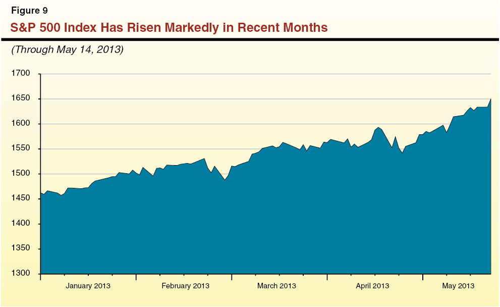
That being said, there is limited evidence to suggest that bubbles currently are widespread in asset markets. Corporate earnings have grown strongly in recent years and have appropriately pushed stock prices upward. As of May 14, for example, the price–to–earnings ratio of the S&P 500 stock index was about 19–to–1. By contrast, the ratio rose to 34–to–1 in 1999 during the “dot–com” bubble, and the mean ratio over a long period has been about 15.5–to–1. The S&P 500 price–to–“book value” ratio was about 2.5–to–1, which is comparable to historical averages and well below the comparable ratio in 2000 (during the dot–com bubble). Potential bubbles in commodities such as silver and gold recently have burst, with little apparent economic impact. House prices are rising, but only after they fell sharply in many regions several years ago. To some extent, the recent rise in stock prices may be influenced by bond yields that have been kept low by accommodative monetary policy, but as a consequence of the various weaknesses in the economy described above, this monetary policy is likely to continue at least into 2014 and thereafter be altered only gradually.
These facts suggest limited evidence of a significant, current bubble in stock and other asset markets. Accordingly, we are utilizing assumptions for future stock market growth in this forecast that are consistent with those used in prior LAO revenue forecasts. As discussed below, capital gains driven largely by stock market trends are a major factor in forecasting California’s revenues. In fact, our statistical models indicate that changes in stock and property prices have accounted for about 80 percent of the annual changes in capital gains. Due to the strength of the relationship between stock prices and this important state revenue source, every California state budget forecast explicitly or implicitly reflects some assumption about the future direction of the stock market.
Role of Capital Gains in California’s Budget. Capital gains are a significant, but volatile, component of California’s PIT revenues. In most recent years, 40 percent to 50 percent of PIT revenues have been paid by the 1 percent of California tax filers with the most income (as of 2011, those tax returns with over $1.4 million of adjusted gross income). Capital gains are a large portion of these taxpayers’ income, and their income tax liabilities attributable to capital gains vary widely from year to year, principally based on trends in prices of stocks and property. In the last decade, income taxes paid by individuals on their capital gains have totaled as little as $2.6 billion in 2009 (about 3 percent of all General Fund revenues) and as much as $12 billion in 2007 (about 12 percent of General Fund revenues).
While Accelerations Were a Factor, Other Causes for Revenue Surge Remain Unclear. The role of capital gains in the state budget recently was highlighted by the influx of $4.5 billion of unanticipated revenues between January and April. While accelerations of capital gains from 2013 to 2012 certainly were one factor behind the revenue surge, the reasons for the bulk of the tax surge remain unclear. Solid data on capital gains and other income reported on 2012 tax returns will take months to compile, which means that forecasters currently have to make various assumptions based on limited data.
Prior forecasts of both our office and DOF already assumed significant accelerations of capital gains realizations from 2013 to 2012. In our prior forecasts, both the LAO and DOF assumed that 20 percent of net capital gains realizations that otherwise would have occurred in 2013 would occur instead in 2012 due to the federal tax changes. In our respective May forecast updates, both of our offices have increased this acceleration assumption. The DOF forecast now assumes that 25 percent of 2013 capital gains realizations were accelerated, and our forecast now assumes that 28 percent were accelerated. These accelerations have the effect of increasing near–term revenue collections, while eroding future revenue collections.
Nevertheless, neither of our updated forecasts seems to adopt the thesis that a large portion of the $4.5 billion tax surge was related to increased accelerations. By increasing the acceleration factor in its forecast from 20 percent to 25 percent, we can make a rough estimate that DOF implicitly assumes that around $2 billion of total accelerated tax payments were received, which is only about $400 million more than the accelerations already reflected in the Governor’s budget forecast in January. Our office’s forecast—with its higher overall capital gains assumptions and a change in the acceleration factor to 28 percent—assumes that around $2.9 billion of total acceleration tax payments were received, which is about $1.2 billion above the level already assumed in the January administration forecast. In short, both of our forecasts suggest that higher capital gains accelerations caused only a part of the $4.5 billion revenue surge of recent months.
Our forecasts’ capital gains assumptions for this year are based on limited data. Similarly, data is not yet available to explain the reason for most of the rest of the revenue surge in 2012–13. Such unexplained variances in state tax collections are common. Forecasting revenues in a state with an economy as complex—and a tax system as volatile—as California’s requires making assumptions each year despite these uncertainties. We attempt to make reasonable assumptions based on the often limited data available. In this forecast, for example, we assume some revenue collections related to tax year 2012 will not recur in later years. The PIT revenues generated by one–time transactions related to Facebook’s initial public offering (which we think may have been higher than assumed in the November 2012 and January 2013 budget forecasts) are an example of revenues that will not recur. While Facebook’s initial public offering was definitely a one–time event, other portions of the unanticipated 2012 tax year revenue may actually prove to be recurring. Thus, while it is possible our PIT assumptions will prove to be too optimistic, it is also possible they will prove to be too cautious.
Assumptions for Future Stock Performance in Our Forecast. As of May 14, the S&P 500 index closed at the level of 1650—up from 1426 at the end of 2012. Our capital gains forecast model is built around an assumption for the average daily close of the S&P 500 in each quarter. Our model assumes that these quarterly averages remain close to the May 14 level of the S&P 500 index through the rest of 2013. Thereafter, we assume that the average S&P 500 close in each quarter increases about 0.9 percent—slower than the growth rate for personal income in our forecast. This sort of assumption has been typical in our recent forecasts.
Even accounting for the recent growth in the stock market, our forecast for 2013–14 PIT revenues is $133 million (0.2 percent) less than our PIT forecast for 2012–13. While accelerations may not explain a large portion of the recent tax revenue surge, they remain substantial and are a major cause of this projected, but small, year–over–year net decline in PIT revenue. (The administration’s 2013–14 PIT revenue forecast reflects an even greater drop from 2012–13—down 4.8 percent—due in part to its lower assumptions for capital gains in 2013.)
Assumed Capital Gains in Our Forecast Compared to Historical Levels. Our forecast assumes that net capital gains realizations by Californians totaled $105 billion in 2012 (virtually identical to DOF’s current assumption). In 2013, we assume that the accelerations reduce net capital gains to $74 billion ($15 billion above DOF’s assumption). In 2014, when the accelerations no longer have a significant influence on our model, net capital gains rise to $103 billion ($20 billion above DOF’s assumption). This roughly $20 billion difference persists through the remainder of our forecast period, accounting for the largest share of the difference between our respective PIT revenue forecasts. Our best assessment is that DOF simply assumes lower capital gains realizations than we do in 2013 and beyond—slightly less than the administration’s own forecast assumed in January 2013 and considerably less than the administration’s forecast in January 2012 (a capital gains forecast that, in retrospect, seems to have been reasonably accurate last year). We find the administration’s pessimism surprising given that (1) the administration’s own estimates of 2012 capital gains are stronger than they were a few months ago (both with and without assumptions regarding capital gains accelerations) and (2) the stock market is much higher than it was in January.
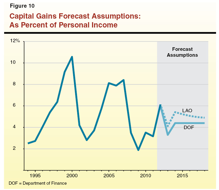
Our capital gains assumptions seem consistent with historical averages for this very volatile part of the taxable income base. Figure 10 shows capital gains as a percentage of California personal income since 1994. From 1994 through 2011, Californians’ capital gains have averaged 5.2 percent of personal income. On average, our forecast assumes that capital gains equal 5.1 percent of personal income between 2012 and 2018 (compared to 4.5 percent in DOF’s forecast). The administration’s economic forecasters also compare capital gains to California GDP. From 1994 through 2011, capital gains have averaged 4.4 percent of California GDP. On average, our forecast assumes that capital gains equal 4.3 percent of California GDP between 2012 and 2018 (compared to 3.8 percent in DOF’s forecast).
Capital Gains and Stock Market Will Be Volatile and Make Budgeting More Difficult. Our model assumes a fairly modest, “straight–line” growth rate for stock prices and annual capital gains totals in line with historical averages. We acknowledge, however, that capital gains and the resulting PIT revenues will not exhibit a straight–line trend in the future. Instead, capital gains and these tax revenues will be volatile. That is, it is likely that capital gains–related taxes will exceed our forecasts in some years and fall short in other years—sometimes by billions of dollars. This complicates the work of the state’s elected leaders in a number of ways. First, it means that each annual budget has to be passed without knowing whether the subsequent year will be a “good” capital gains year or a “bad” one. In the latter circumstance, the fiscal year can close with a shortfall, necessitating budget cuts or other budget actions in the ensuing year. Second, the volatility of capital gains makes it very difficult to plan for the state’s annual level of required school spending under Proposition 98, given that Proposition 98 is affected significantly by the year–over–year growth rate in state General Fund revenues. These challenges are only increasing due to Proposition 30, recent decisions about how to make Proposition 98 maintenance factor payments, and the state’s recently adopted revenue accrual policies. (The nearby box discusses those accrual policies.)
2011–12 Revenues Will Continue to Evolve. The state’s 2011–12 fiscal year “ended” over ten months ago, but the May Revision decreases the estimates of state revenues for that fiscal year by $285 million. Under the state’s new revenue accrual approach for Proposition 30 and Proposition 39 revenues, a portion of collections for 2012 were “accrued back” to 2011–12. The 2011–12 revenue amount will continue to change until 2014 or even longer because solid data on what the state collected in 2012 tax revenues will take many months to compile. This practice is slated to continue in the administration’s budget plan. More 2013 tax collections than are actually collected prior to June 30, 2013 will be accrued back to the current fiscal year, and so on, for each year that the policy remains in place. These accruals are difficult for revenue forecasters to predict and add to the already substantial possibility of error in state budget revenue forecasts.
Not Knowing Last Year’s Revenues Complicates Budgeting. As anyone who reads this publication’s Proposition 98 description will see, the amount of revenues in each specific year determines not only how much money is available for state spending, but also how much must be spent on schools. It is becoming increasingly unmanageable for policymakers to set each year’s state budget plan without a clear idea of how both the current and prior fiscal years ended.
Current Accrual Policies Diminish Legislative Authority. The current accrual process—for all revenues, including Propositions 30 and 39—lacks transparency. Executive branch officials seem to have broad flexibility concerning the fiscal year to which each revenue dollar is assigned. This, in turn, could allow a Governor to increase or decrease the Proposition 98 guarantee as he or she sees fit. Moreover, in the rare fiscal year like this one (in which the current method for paying Proposition 98 maintenance factor is absorbing more than every dollar of increased revenue), continuing to accrue next fiscal year’s cash into the current fiscal year results in the Legislature having less flexibility to set its own budgetary priorities.
Recommend Transitioning to Simpler Accrual Policy. Returning state budgetary revenue accounting to something approximating a cash basis—counting revenues in the fiscal year in which they are collected—would correct these problems. A multiyear transition plan is required, which, by its nature, will result in the Proposition 98 minimum guarantee being more or less in the years during the transition. We recommend that the Legislature direct the administration to submit a multiyear plan for a return to a transparent, logical, and simpler budgetary revenue accrual policy.
Caution Is Appropriate Concerning Capital Gains. Caution is in order for the state’s elected leaders. No matter which revenue assumptions are used in the budget, there is a risk that revenues will end up considerably lower than projected. (Obviously, there is a greater risk of this if the state uses our office’s higher revenue projections for the 2013–14 budget plan.) There is also a chance that revenues will end up higher than expected, even compared to our office’s forecast. In the end, revenues will differ from estimates one way or another—perhaps by billions of dollars. Our office attempts to take our “best shot” at making a projection with the release of each state revenue forecast. With regard to capital gains, our projections seem to us to be neither too cautious nor too optimistic based on the recent status of financial markets.
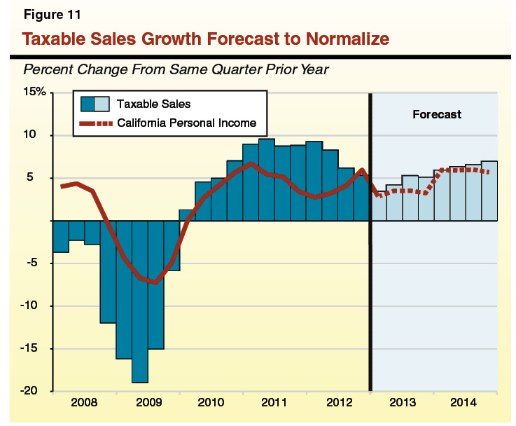
Lower Sales Tax Forecast in 2013–14. Our forecast assumes slightly higher General Fund SUT collections than the administration in 2012–13 but is $789 million lower than the administration for 2013–14. Taxable sales in California—the main determinant of SUT revenue—declined substantially during the recession as consumers and businesses delayed major purchases, especially of vehicles, industrial equipment, and household appliances. Since that time, taxable sales have grown briskly from their historically depressed levels—with taxable sales growth rates exceeding the growth of personal income in the state, as shown in Figure 11 (see page 20). In prior forecasts, our office has noted that the annual growth in taxable sales should revert to more normal levels over time as consumers and businesses return to typical consumption patterns. In recent months, actual taxable sales growth has been markedly slower than our most recent estimates, leading both our office and the administration to revise downward 2012–13 General Fund SUT estimates. The administration essentially projects that this downward trend will reverse itself for a time (DOF projects taxable sales to grow by more than 8 percent in 2013–14), whereas we think that taxable sales growth has begun to normalize, resulting in our lower (5 percent annual growth) growth expectation for 2013–14.
Corporate Income Taxes Remain Difficult to Project. Currently, our forecast for CT revenues is similar to that of the administration. Both of our forecasts anticipate hundreds of millions of dollars less in CT revenues in 2013–14 compared to the January 2013 administration forecast. Nevertheless, we caution, as we have for some time now, that this tax remains very difficult to predict, given the wide array of recent CT policy changes adopted by the state (the estimated effects of which remain somewhat unclear) and other recent developments. Among those recent developments has been a marked increase in CT refunds in 2012–13—up 51 percent from the prior fiscal year through April. We understand that a portion of this higher refund activity relates to the resolution of certain large business tax disputes by the Franchise Tax Board, and this refund activity in turn has resulted in a larger amount of CT refunds accrued to the prior fiscal year (2011–12). These accrual developments are responsible for a part of the administration’s $716 million reduction of its 2011–12 CT forecast. Our forecast assumes that further such refund activity continues in the coming months. Moreover, our forecast reflects some degree of caution due to the weak results for April 2013 estimated payments by corporations, which were 1 percent below those of April 2012. In the coming months, a particularly important new set of data we will have to consider will be the level of net operating loss deductions claimed by larger California businesses in 2012, the first year they can use these deductions after they were prevented from claiming them for a few years during the budget crisis. Higher or lower levels of these deductions in 2012 could affect future forecasts by hundreds of millions of dollars per year.
Administration’s Business Tax Proposal. The administration’s May Revision submissions to the Legislature include a proposal—described by the administration as “revenue neutral”—to change certain business tax provisions. The proposal lacks some key details, but seems to be focused on shrinking over time the scale of parts of California’s existing enterprise zone tax program. The proposal, as we understand it, also would eliminate the state General Fund portion of the sales tax on certain manufacturing and biotechnology equipment, change a state hiring tax credit (which was little used during the recession), and establish a “recruitment and retention” fund that the Governor’s Office of Business and Economic Development would administer to grant tax credits to businesses that meet certain jobs–related criteria. Our revenue forecast assumes, based on the administration’s stated goals, that the plan, if adopted, would be revenue neutral through at least 2017–18. In reality, it will be very difficult for the administration to design an approach that is precisely revenue neutral in future years.
Our initial impression is that there are some positive parts of this proposal—specifically, as we understand it, scaling back the ineffective enterprise zone program and reducing certain manufacturing sales taxes. (Such taxes are one of a number of state tax provisions that create “tax pyramiding”—an economically distortionary phenomenon whereby businesses pay sales tax on their equipment and their customers then pay additional sales tax on the final product itself.)
On the other hand, we are skeptical that the hiring credit and incentive fund can be designed in ways that achieve their stated goals without providing windfall gains to businesses for decisions they would have made even without the tax incentives. In general, we advise the Legislature to move toward state tax changes that spread the cost of public services over the broadest base possible, with fewer tax expenditures focused on select segments of the economy. By doing this, the state would have the option of lowering certain marginal tax rates and yet be able to collect approximately the same amount of tax revenue.
Approved by voters in 1988, Proposition 98 established a set of rules relating to education funding. Most importantly, Proposition 98 established a funding requirement commonly referred to as the minimum guarantee. The minimum guarantee is determined by various inputs (including General Fund revenues and K–12 average daily attendance) and formulas (including calculations that compare growth in per capita General Fund revenues with growth in per capita personal income). The guarantee is funded with state General Fund revenues and local property tax revenues. Funding provided for schools, the California Community Colleges (CCC), preschool programs, and various other state education programs count toward meeting the guarantee. This section of the report describes and assesses the Governor’s May Revision Proposition 98 proposals.
Proposition 98 Funding Changes Significantly in May Revision. Shown in Figure 12, the 2012–13 minimum guarantee under the May Revision is $56.5 billion—almost $3 billion higher than the January level. Virtually the entire increase reflects higher General Fund costs, with updated 2012–13 local property tax estimates almost identical to the January estimates. Whereas the guarantee in 2012–13 is notably higher, the guarantee in 2013–14 is notably lower. The 2013–14 minimum guarantee under the May Revision is $55.3 billion—down almost $1 billion from the January level. Because the updated 2013–14 local property tax estimate is significantly higher than the January estimate (up $579 million), the General Fund Proposition 98 cost for 2013–14 is estimated to be $1.5 billion lower than the January estimate. As discussed in more detail later in this section, almost the entire change in the guarantee for these two fiscal years is driven by changes in state revenues, with updated estimates of student attendance in 2012–13 and 2013–14 up only slightly from the January estimates.
Figure 12
Proposition 98 Funding
(In Millions)
|
|
2012–13
|
|
2013–14
|
|
January
|
May Revision
|
Change
|
|
January
|
May Revision
|
Change
|
|
Preschool
|
$481
|
$481
|
—
|
|
$481
|
$482
|
—
|
|
K–12 Education
|
|
|
|
|
|
|
|
|
General Fund
|
$33,406
|
$36,196
|
$2,790
|
|
$36,084
|
$35,028
|
–$1,057
|
|
Local property tax revenue
|
13,777
|
13,773
|
–5
|
|
13,160
|
13,668
|
508
|
|
Subtotals
|
($47,183)
|
($49,968)
|
($2,786)
|
|
($49,244)
|
($48,696)
|
(–$548)
|
|
California Community Colleges
|
|
|
|
|
|
|
|
General Fund
|
$3,543
|
$3,699
|
$157
|
|
$4,226
|
$3,761
|
–$464
|
|
Local property tax revenue
|
2,256
|
2,253
|
–3
|
|
2,171
|
2,242
|
71
|
|
Subtotals
|
($5,799)
|
($5,953)
|
($153)
|
|
($6,397)
|
($6,003)
|
(–$393)
|
|
Other Agencies
|
$78
|
$78
|
—
|
|
$79
|
$78
|
–$1
|
|
Totals
|
$53,541
|
$56,480
|
$2,939
|
|
$56,200
|
$55,259
|
–$941
|
|
General Fund
|
$37,507
|
$40,454
|
$2,947
|
|
$40,870
|
$39,349
|
–$1,521
|
|
Local property tax revenue
|
16,034
|
16,026
|
–8
|
|
15,331
|
15,910
|
579
|
Changes in Guarantee Linked With Notable Changes in Proposition 98 Spending. Figure 13 shows the May Revision changes in Proposition 98 spending. Of the $2.9 billion increase in the 2012–13 guarantee, the Governor designates $1.8 billion for paying down additional deferrals, $1 billion for a new initiative to help school districts implement the Common Core State Standards (CCSS), and the remainder for various relatively small baseline adjustments mostly associated with changes in revenue limit costs. Of the $941 million decrease in the 2013–14 guarantee, the Governor reduces the amount of deferral pay downs and rescinds most of his January community college proposals. These actions reduce spending by a total of $1.5 billion, thereby freeing up about $600 million for other Proposition 98 purposes. The Governor directs the bulk of the $600 million to the Local Control Funding Formula (LCFF), various new community college proposals, and backfilling the federal sequestration cut to special education. The May Revision also includes a revised estimate of Proposition 39 corporate tax revenues, resulting in a small increase ($14 million) in energy–related funding for schools and community colleges. We discuss several of these spending proposals in more detail later in this section.
Figure 13
Proposition 98 May Revision Spending Changes
|
|
|
|
2012–13 Changes:
|
|
|
Pay down additional deferrals
|
$1,783
|
|
Fund one–time Common Core implementation initiative
|
1,000
|
|
Make technical adjustments
|
156
|
|
Total
|
$2,939
|
|
2013–14 Changes:
|
|
|
Reduce deferral paydown
|
–$1,024
|
|
Rescind January adult education proposal
|
–300
|
|
Rescind January CCC unallocated base augmentation
|
–197
|
|
Swap additional one–time funds
|
–22
|
|
Provide additional funds for Local Control Funding Formula
|
240
|
|
Fund CCC enrollment growth
|
89
|
|
Provide cost–of–living adjustment to CCC apportionments
|
88
|
|
Backfill special education sequestration cut
|
61
|
|
Fund CCC student–support program
|
50
|
|
Make technical adjustments
|
31
|
|
Fund adult education planning grants
|
30
|
|
Increase funds for Proposition 39 energy projects
|
14
|
|
Total
|
–$941
|
Changes in Programmatic Per–Pupil Funding Offer Different Perspective. Under the May Revision, K–12 programmatic per–pupil funding is $7,588 in 2012–13—roughly the same as under the January plan and flat from the prior year. Because the increase in 2012–13 spending under the May Revision is designated for paying down deferrals and the new CCSS initiative to be implemented in subsequent years, the programmatic impact in the current year is assumed to be negligible. In 2013–14, programmatic per–pupil funding under the May Revision is $8,081—$152 higher than the January level and $493 (6 percent) higher than the current year. This increase is largely associated with the additional funding provided for the LCFF. Our estimates also assume that schools would spend half of the CCSS funding for programmatic purposes in 2013–14 (with the remainder spent in 2014–15). At CCC, programmatic funding per full–time equivalent (FTE) student increases under the May Revision by 4 percent, from $5,418 in 2012–13 to $5,638 in the 2013–14
Revenue Estimates Result in Significant Increase in 2012–13 Proposition 98 Minimum Guarantee. The May Revision estimates of General Fund revenues that count toward the minimum guarantee are roughly $300 million lower in 2011–12 and $2.9 billion higher in 2012–13 relative to the January estimates. The current–year minimum guarantee increases roughly $1.1 billion as a result of higher total 2012–13 General Fund revenues. The minimum guarantee also increases because of the change in the year–to–year growth in revenues. The combination of a decrease in 2011–12 and an increase in 2012–13 significantly increases year–to–year General Fund growth and results in a larger 2012–13 Proposition 98 maintenance factor payment ($4.4 billion, an increase of $1.8 billion from the January estimate). Taken together, these two factors explain the $2.9 billion increase in the 2012–13 minimum guarantee under the May Revision.
Revenue Estimates Result in Notable Drop in 2013–14 Proposition 98 Minimum Guarantee. The May Revision estimate of General Fund revenues that count toward the guarantee in 2013–14 is $1.8 billion lower than the January estimate. Given the notable increase in 2012–13 revenues and the decline in 2013–14 revenues, the year–to–year growth rate drops significantly. This drop in year–to–year revenue growth results in a $1 billion reduction in the minimum guarantee. This reduction is offset by a small increase ($106 million) due to updating various other inputs, including K–12 attendance (projected to grow by 0.20 percent, up from 0.10 percent in January). Combined, these changes explain the net $941 million decrease in the 2013–14 minimum guarantee under the May Revision.
“Spike Protection” Provision Dampens the Ongoing Effect of Large Current–Year Increase in Minimum Guarantee. Under the May Revision, General Fund revenues that count toward the guarantee in 2013–14 ($95.2 billion) are somewhat higher than 2012–13 ($94.6 billion). The minimum guarantee, however, is lower in 2013–14 ($55.3 billion) than 2012–13 ($56.5 billion). This rare situation is due to the spike protection provision of Proposition 98. (2013–14 would be the first time this provision has ever taken effect.) In a year when the minimum guarantee increases at a much faster rate than per capita personal income, the spike protection provision excludes a portion of Proposition 98 funding from the minimum guarantee calculation in the subsequent year. In the May Revision, the spike protection provision excludes $1.5 billion in 2012–13 Proposition 98 funding from the 2013–14 Proposition 98 calculations, reducing the 2013–14 minimum guarantee by a like amount. Although the spike protection provision also was applied in the Governor’s January budget, the effect was much smaller ($279 million).
Estimates of Proposition 98 Local Property Tax Revenues Up Notably. Estimates of Proposition 98 local property tax revenues are up a total $736 million across the three–year period under the May Revision (up $165 million in 2011–12, down $8 million in 2012–13, and up $579 million in 2013–14). The increase in 2011–12 is primarily due to increases in base property tax revenues. In 2013–14, property tax revenues are up mostly due to higher estimates of redevelopment agency revenues that will be redirected to schools and community colleges. The higher property tax estimates for schools and community colleges generally result in a dollar–for–dollar reduction in state General Fund Proposition 98 costs.
One–Time Funding for Implementing CCSS. California adopted the nationally developed CCSS in 2010 and, pursuant to federal direction, is planning to begin implementing the new standards in the 2014–15 school year. One way the May Revision responds to the large increase in the current–year guarantee is by providing $1 billion to school districts on a one–time basis for implementing the CCSS. The May Revision proposes to allocate this funding on a per–student basis (equating to about $170 per student). School districts would be required to use the funds for instructional materials, professional development, or technology related to CCSS implementation. Districts would need to develop a related expenditure plan and spend the funds over the next two years (2013–14 and 2014–15). The CCSS spending would be subject to the annual funding and compliance audit.
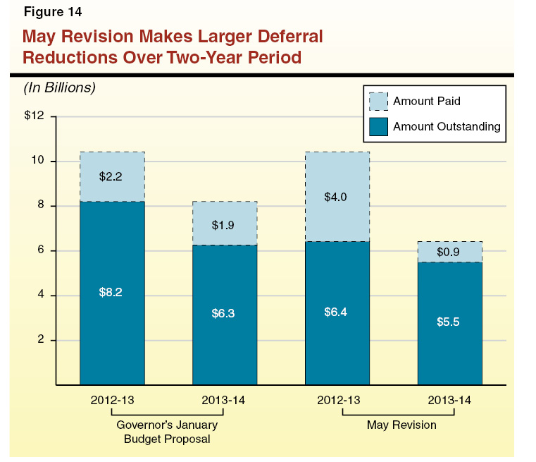
Increases Deferral Paydowns Over Two–Year Period. Figure 14 shows the changes in the Governor’s proposal to reduce the amount of outstanding K–14 payment deferrals. The May Revision provides an additional $1.8 billion to retire existing deferrals in 2012–13—for a total current–year paydown of $4 billion. As a result of the decline in the minimum guarantee in 2013–14, the Governor reduces his proposed 2013–14 paydown by almost $1 billion (to $920 million). Compared to the January proposal, the May Revision retires an additional $760 million in deferrals over the two–year period, leaving $5.5 billion in outstanding deferrals at the end of 2013–14.
Makes Some Modifications to LCFF, Increases Year–One Funding. In January, the Governor proposed to replace the state’s existing system for allocating funding to school districts and charter schools with a new student–based funding formula. The May Revision proposes an additional $236 million for implementing this formula (bringing total 2013–14 funding for LCFF implementation up to $1.9 billion). The Governor also makes various modifications mostly relating to the proposed funding supplement for English learners and low–income (EL/LI) students, including: (1) basing EL/LI counts on a three–year rolling average, (2) allowing EL students to generate supplemental funding for seven (rather than five) years, and, (3) requiring districts to allocate EL/LI funding to school sites in proportion to their enrollment of EL/LI students. Additionally, the Governor proposes to strengthen academic accountability by developing a tiered intervention system through which county superintendents, the Fiscal Crisis and Management Assistance Team (FCMAT), and Superintendent of Public Instruction (SPI) could intervene in districts failing to meet academic performance targets. (The May Revision makes no major modifications to the proposed LCFF for county offices of education [COEs] but provides an additional $4 million in funding—on top of the $28 million proposed in January.)
Introduces New Proposal for Adult Education. The Governor rescinds his January proposal that would have provided CCC with $300 million in base funding for adult education. Instead, the May Revision proposes to provide $30 million in the budget year for community colleges and school districts (through their adult schools) to create joint plans for serving adult learners in their area. Providers would have two years to form regional consortia and develop plans for coordinating and integrating services. Beginning in 2015–16, the administration proposes to provide $500 million to the regional consortia to deliver adult education. Under the administration’s plan, each consortium would submit an application to the California Department of Education (CDE) and CCC Chancellor’s Office, which would jointly review the applications and allocate the funding. Funding would be limited to core adult education programs (such as English as a second language and vocational instruction) and all providers would receive the same enhanced noncredit funding rate that community colleges receive. To create an incentive for school districts (as well as community colleges) to maintain existing levels of support for adult education over the next two years (2013–14 and 2014–15), the Governor proposes to earmark two–thirds of the proposed $500 million augmentation in 2015–16 for providers that meet this criterion.
Substitutes Unallocated Base CCC Increases for Targeted Augmentations. The Governor also rescinds his January proposal to provide an unallocated base increase to CCC of $197 million. Instead, the May Revision provides a total of $227 million to CCC for three specific purposes: (1) funding 1.63 percent enrollment growth ($89 million), (2) providing a 1.57 percent cost–of–living adjustment (COLA) for apportionments ($88 million), and (3) augmenting the Student Success and Support categorical program (formerly known as Matriculation), which funds services such as orientation and counseling ($50 million).
Allocates $61 Million to Backfill Federal Sequestration Cut to Special Education. California’s federal Individuals with Disabilities Education Act (IDEA) grant is projected to be cut $61 million as a result of sequestration. In contrast to the other education sequestration cuts (including an $84 million drop in Title I support for students from low–income families), the May Revision would backfill this loss with ongoing Proposition 98 funds. Most of the proposed backfill would be distributed based on the state’s “AB 602” allocation formula. (A small amount—$2.1 million—would be dedicated to special education infant/toddler and preschool services.) The $61 million equates to about 1 percent of total special education categorical funding.
Most New Revenue Dedicated to Proposition 98 Because of Maintenance Factor Application. The changes in the Proposition 98 minimum guarantee stemming from updated General Fund revenue estimates have resulted in highly unusual outcomes whereby schools and community colleges have disproportionately benefited from improvements in General Fund revenues. These outcomes are driven by the Governor’s approach to calculating maintenance factor payments in Test 1 years (2012–13 is a Test 1 year). The Governor’s maintenance factor treatment ratchets up the minimum guarantee, such that the $2.8 billion increase in 2012–13 General Fund revenues in the May Revision results in a $2.9 billion increase in the minimum guarantee. This result essentially requires the state to make budget reductions in other areas to pay for additional Proposition 98 costs. We question the reasonableness of an approach that results in the rest of the budget under certain situations not benefitting at all from revenue growth.
LAO Option Frees Up Almost $3 Billion. If the state were to use an alternative interpretation of maintenance factor—one akin to the past interpretation in which about 50 percent to 55 percent of revenue growth went to K–14 education—the budget situation facing the state would be quite different. Using this alternative application, the minimum guarantee in 2012–13 would be $53.6 billion. This is $2.9 billion below the May Revision estimate but almost identical to the Governor’s January estimate, meaning that the state could keep the existing current–year spending plan. In 2013–14, the minimum guarantee ($53.8 billion) would be lower than the January and May Revision levels, but the Legislature could provide more than the minimum guarantee and fund at whatever level it chose. If the Legislature chose to spend at the 2013–14 May Revision Proposition 98 level, it still would have $2.9 billion available—funds that could be used to build up the budget reserve, pay off debts, or spend on non–Proposition 98 programs. Alternatively, if the Legislature chose to spend at the higher January Proposition 98 level, it would have $1.9 billion available. The Legislature could choose to fund Proposition 98 even higher than the January level, determining how much of the $1.9 billion to leave for other priorities. Such an approach offers the Legislature considerably more flexibility in building the 2013–14 state budget.
Mix of One–Time and Ongoing Spending Reasonable. We believe the May Revision approach of using new one–time 2012–13 funds for one–time initiatives (including the acceleration of deferral pay downs) is prudent. We also think the May Revision 2013–14 approach of dedicating about one–quarter of new resources to paying down deferrals and the remainder to building up ongoing programmatic spending is reasonable. Although the Governor dedicates a smaller share of new resources in 2013–14 to paying down existing obligations under the May Revision compared to the January plan, the May Revision pays down more deferrals across the two–year period. Though the state will face a somewhat greater challenge in 2014–15 in finding available resources to continue paying down deferrals given this approach, the amount of total outstanding deferrals will be lower by $760 million moving into 2014–15.
One–Time Common Core Implementation Initiative Raises Important Issues to Consider. The Legislature has several important issues to consider regarding how best to spend an additional $1 billion in one–time funding. The Legislature faces significant trade–offs in deciding whether to use the funding for CCSS implementation or other existing one–time obligations. For example, the Legislature could use the funds to pay down additional deferrals, pay outstanding mandate claims, retire more of the Emergency Repair Program obligation (an obligation relating to a legal settlement), or fund other activities, such as facility maintenance, that have been reduced significantly over the past several years. Were the Legislature to deem CCSS implementation the highest of these priorities, it then would want to consider both how much to provide and what requirements, if any, to link with the funding. As part of this decision making, the Legislature would want to consider the amount of existing local, state, and federal resources that can be used to cover CCSS implementation costs, such that the additional amount of state resources provided could cover otherwise unaddressed implementation costs.
Overall LCFF Framework Remains Sound. We continue to believe that the overarching structure of the Governor’s LCFF proposal is sound and recommend the Legislature adopt some variant of it. We believe most of the specific LCFF modifications proposed in the May Revision are reasonable but likely would have only a minor effect on districts and their funding allotments. In a few cases (such as the new requirements related to school–site expenditures), we are concerned that the modifications in the May Revision could limit districts’ flexibility and increase their administrative burden. The Governor’s May Revision proposal relating to academic accountability under the LCFF seems generally reasonable in that it attempts to outline certain steps county superintendents, FCMAT, and the SPI can take to intervene in struggling districts. This proposal somewhat parallels existing practices for holding districts fiscally accountable. We have some concerns, however, regarding the current capacity of the county superintendents, FCMAT, and the SPI to perform these duties effectively. As the Governor proposes to begin implementing the new system in 2015–16, we think the Legislature could take some more time to consider the specific roles of each identified agency and then accordingly build their capacity to advise, support, and intervene in struggling districts.
Recommend Governor’s COE Proposal Be Postponed One Year. As described in our January report, we have serious concerns with the Governor’s proposal for COEs. Specifically, the proposal: (1) increases funding for regional services while reducing the responsibilities of COEs, (2) compounds the existing lack of accountability over how COEs spend regional funding, and (3) increases alternative education funding by up to $7,000 per student without clear justification. Given these concerns and the short amount of time remaining this budget season to address them, we recommend the Legislature retain the existing COE funding formulas in 2013–14 and refine the Governor’s proposal during the upcoming year. This alternative would allow the state additional time to consider carefully what activities should be required of all COEs and develop an appropriate funding rate for those activities beginning in 2014–15. If the Legislature were to adopt this recommendation, $32 million would be freed up for other Proposition 98 purposes in 2013–14.
Promising Plan for Adult Education. We believe the May Revision adult education proposal is much better than the Governor’s January proposal. By proposing a regional delivery model, the new plan would create a strong incentive for adult–education providers to leverage their relative strengths and improve collaboration. By conditioning the bulk of new base funding on providers maintaining at least their current level of service, the May Revision also would create an incentive for providers to continue offering adult education programs in 2013–14 and 2014–15. We think the two–year planning time frame is reasonable. During this preparation period, providers would have an opportunity to identify program needs and create aligned curricula. At the same time, the Legislature, CDE, and the CCC Chancellor’s Office could be addressing state–level issues in support of the regional consortia, such as developing a common course numbering system for adult education and deciding on the amount of funds each region would be eligible to apply for beginning in 2015–16. While we agree with the overall approach proposed by the Governor, we recommend the Legislature provide more flexibility for providers to organize themselves (for example, by allowing the Chancellor’s Office to pass through funds to school districts if they are interested in being a consortium’s fiscal agent).
Proposed CCC Base Augmentations Have Merit. In our analysis of the Governor’s January proposal to provide an unallocated increase to CCC, we voiced serious concern that such an approach would provide no assurance that the Legislature’s priorities would be met. The May Revision addresses this concern by funding specific and high legislative priorities such as access (enrollment) and student support services. As such, we recommend the Legislature approve the administration’s May Revision proposal.
Special Education Backfill Proposal Is Reasonable. We believe the Governor’s proposal to increase Proposition 98 spending for special education is reasonable. Though the state is not obligated to backfill this cut in federal funding, school districts are required by federal law to provide special education services and a reduction in federal funding likely would lead to an increase in the amount of local general purpose funds school districts would have to dedicate for these services. This likely would exacerbate a recent trend in which school districts appear to be bearing a greater share of special education costs, as growth in state categorical and federal IDEA funds have not been keeping pace with growth in special education costs over the last several years.
General Fund Proposition 98 Costs Higher Than Estimated in May Revision. The Governor’s May Revision fails to recognize additional General Fund Proposition 98 costs related to the allocation of Education Protection Account (EPA) funds. Proposition 30 requires that each school district receive at least $200 in EPA funds per student and each community college district receive at least $100 per FTE student. For most districts, EPA funds will be used to pay for costs that otherwise would have been paid with state General Fund dollars. As a result, those EPA allocations will not increase state costs. Some districts, however, do not receive base state funding because associated costs can be met entirely with their local property tax revenues. For these districts—known as basic aid districts—EPA allocations will result in higher state costs. The May Revision does not account for these costs. We estimate the annual cost in 2012–13 and 2013–14 at $68 million ($62 million for school districts and $6 million for community college districts). We recommend the Legislature include these costs in building its Proposition 98 budget package and reduce spending in other Proposition 98 programs to maintain spending at the minimum guarantee in both 2012–13 and 2013–14.
Under the ACA, also known as federal health care reform, the state has the option to expand its Medicaid Program (known as Medi–Cal) to cover over one million low–income adults who are currently ineligible. For three years, beginning January 1, 2014, the federal government will pay almost all the costs associated with the expansion. Beginning January 1, 2017, the federal share of costs associated with the expansion would be decreased over a three–year period until the state pays for 10 percent of the expansion and the federal government pays the remaining 90 percent. Currently, the counties have the fiscal and programmatic responsibility for health care for the low–income adult population that would be covered by the expansion (hereafter referred to as the expansion population).
Adopts the Optional Medi–Cal Expansion Using a State–Based Approach. In January, as we discussed further in our report,
The 2013–14 Budget: Examining the State and County Roles in the Medi–Cal Expansion, the Governor proposed to adopt the optional Medi–Cal expansion and proposed two options to implement the expansion: (1) a county–based approach or (2) a state–based approach. The Governor’s May Revision proposes to adopt a state–based approach under which the state would expand its existing state–administered Medi–Cal Program to cover the expansion population. The expansion population would receive the same set of benefits currently provided by Medi–Cal—including long–term care services if the federal government allows the state to restrict these services to individuals with limited financial assets. Counties would have the option to provide enhanced substance use disorder services to both new and existing enrollees.
Redirects County Indigent Health Funding. Under the proposal, the responsibility for providing health care to the expansion population would shift from counties to the state—resulting in significant savings for counties. The May Revision proposes to redirect certain funding provided to counties for indigent health care under the 1991 state–county realignment plan in order to help cover increased state costs due to the optional expansion and the ACA. (Under the 1991 realignment, the state transferred to counties certain health and human services program responsibilities and offset counties’ expanded fiscal responsibilities with increased sales tax and vehicle license fee revenues.)
The May Revision proposes to establish a mechanism (hereinafter referred to as the “formula”) to calculate annual county health care savings available for redirection. Based on initial discussions with the administration, county health care savings under this formula would be defined as the difference between (1) county health care revenue and (2) county costs for providing services to Medi–Cal beneficiaries (the expansion population and current enrollees) and uninsured patients. The formula includes some adjustments, presumably intended to (1) safeguard resources for county mental health and substance use programs and (2) ensure that the calculation of county savings is not affected by future county actions to redirect health care resources or greatly increase health care spending. These adjustments include:
- County Mental Health and Substance Use Disorder Services Resources Would Be Excluded. The formula excludes resources for mental health and substance use disorder services from its calculations of county health care revenue and spending.
- County Health Care Revenue Estimates Would Be Based Partly on Historic Factors. The formula would include actual federal funds and patient payments provided to counties. The amount of county health care funds attributable to 1991 realignment and local sources, in contrast, would be based on county prior use of these resources for health care purposes.
- High Growth in County Health Care Costs Would Be Excluded From the Formula. The formula would include actual costs experienced by counties during each year of ACA implementation, up to a specified cap based on historical spending levels. Actual county expenditures above the cap would not be incorporated into the formula.
The May Revision estimates that county health care savings under this approach would be $300 million in 2013–14, $900 million in 2014–15, and $1.3 billion 2015–16.
Realigns State and County Responsibilities for Health and Social Services Programs. The administration proposes to redirect these county healthcare savings to pay for increased county costs resulting from a new state–county program realignment. Under the new realignment, counties would assume increased fiscal responsibility for CalWORKs, CalWORKs–related child care, and CalFresh administration—decreasing state General Fund spending in these programs dollar–for–dollar. The state would maintain its current policy making and oversight responsibilities for these programs. Additionally, county fiscal responsibility for California Children’s Services would be shifted to the state. Pending future developments (which the administration has not yet defined), county costs for In–Home Supportive Services also might be shifted to the state. In total, the realignment package is intended to increase county costs by an amount equal to county indigent health savings and decrease state General Fund spending by a corresponding amount.
State–Based Expansion Makes Sense. In our February report examining Medi–Cal expansion, we recommended the Legislature adopt a state–based expansion. The Governor’s proposal is consistent with our recommendation. We believe the state is in a better position than the counties to effectively organize and coordinate the delivery of health services to the newly eligible population—potentially resulting in improved health outcomes and administrative efficiencies. As a practical matter, we also believe the state is better positioned than the counties to successfully implement an expansion by January 1, 2014.
New Realignment Presents Significant Issues. The Governor’s realignment proposal raises two primary concerns. First, the new realignment proposal adds complexity to the already complicated issue of implementing the optional expansion. Evaluating programs as to their suitability for state–county realignment is complex and only should be implemented after thorough deliberation by the Legislature and discussions with the administration, counties, and program stakeholders. For example, in considering the realignment of CalWORKs, the Legislature would need to assess whether it is willing to relinquish some policy making authority over the program and allow variation in treatment of recipients across counties. Given the multitude of issues the Legislature will face in implementing the optional expansion, we suggest the Legislature avoid introducing additional issues—such as complicated shifts of authority over unrelated programs—into discussions of the optional expansion. Second, the realignment proposal raises concerns about potential increased county costs and state mandates. Specifically, under the proposed realignment plan, counties would have increased fiscal responsibility for human services programs. The California Constitution generally requires the state to reimburse local governments if it mandates that local governments provide a new program, pay an increased share of a program’s cost, or provide a higher level of service. Forecasting future costs for caseload–driven programs such as CalWORKs, child care, and CalFresh is very difficult. For this reason, in future years it would be difficult to ensure that the redirected realignment funds were sufficient to cover the costs of new county responsibilities. If funding fell short of what is required to fund the counties’ new responsibilities, counties could experience fiscal pressure and the state could be liable for claims for mandate reimbursements.
Proposed Formula Appears to Diverge From Stated Goals of Financing Expansion. The administration has articulated two major goals in its proposal for financing the optional expansion: (1) to ensure the state no longer funds counties to provide health care to patients who gain Medi–Cal and private coverage under ACA, and (2) to preserve access to county–operated hospitals and clinics for Medi–Cal beneficiaries and the remaining uninsured. While we find the administration’s goals to be reasonable, we note that the formula for determining county savings—as described to us by the administration—appears to diverge from these stated objectives. Specifically, by incorporating in the formula revenues and costs related to all Medi–Cal patients, including currently eligible enrollees, the mechanism would define county healthcare savings to encompass a broader patient population than the formerly indigent. In our view, redirecting net county savings from all payer sources is a distinct concept from preventing overpayments from realignment funds for the formerly indigent. Furthermore, the state’s claim to all county health care funds in excess of the formula’s calculations of their health care costs may limit incentives and resources for counties to reinvest in county public hospitals and clinics.
Basis for County Savings Estimates Is Unclear. At the time this report was written, the methodology and assumptions used by the administration to estimate county savings were unclear. Additionally, as we discussed in our February report, data on county indigent health expenditures are limited. According to the administration, information about county indigent health costs submitted to the state as part of the Medi–Cal Section 1115 waiver—including Low–Income Health Program cost information—was a primary source of information used to estimate county savings. While we believe this cost information could be useful in estimating county savings, the information has some significant limitations—such as the fact that not all counties operate a Low–Income Health Program.
The Governor’s proposal raises concerns in that it: (1) unnecessarily ties implementation of the optional expansion to a complicated new state–county realignment and (2) appears to rely on a formula for calculating expansion–related savings that does not square with the administration’s stated principles. Below, we discuss an alternative that attempts to address these concerns.
Redirect Realignment Funds Historically Related to Expansion Population. Under our alternative, the Legislature would redirect the share of 1991 health realignment funds historically associated with providing services to the expansion population—about 46 percent of total health realignment funds. (We discuss the policy basis for this redirection in our February report.) Accounting for the partial–year implementation of the optional expansion in 2013–14, this approach would suggest redirecting about $325 million in that fiscal year. However, in light of the uncertainty surrounding the implementation of the optional expansion and the potential administrative difficulties that may arise, the Legislature may want to consider redirecting a somewhat lesser amount—perhaps $300 million, as suggested by the Governor—in 2013–14. In 2014–15 and 2015–16, the amount redirected under this approach would be around $700 million.
Establish a Review Process to Protect Solvency of Public Hospitals and Clinics. The Legislature could create a process to formally review the solvency of public hospitals and clinics to ensure the above described shift of 1991 realignment funds does not threaten the financial viability of safety–net providers. This process would involve various state and county stakeholders and review data on actual county funding and costs for the operation of public hospitals and clinics as it becomes available. The findings of this review could be presented to the Legislature and used to adjust the amount of redirected realignment funding in future years.
Use Indigent Health Realignment Funds to Pay Some CalWORKs Costs. Instead of making major changes to county fiscal and program responsibilities as proposed by the Governor, the Legislature could build upon an existing arrangement created under the 2011 realignment plan (a recent state–county realignment that, among other changes, transferred responsibility for certain criminal offenders from the state to counties) that uses county funding to offset state General Fund costs for CalWORKs grants. Under this approach, redirected indigent health realignment funds would be placed in an account within the 1991 realignment structure to help pay for CalWORKs grant costs—creating dollar–for–dollar state General Fund savings. This approach does not fundamentally increase county financial responsibility for supporting CalWORKs and does not change the state’s authority over or programmatic responsibility for CalWORKs. As a result, it would be a much simpler approach to implement—particularly in the near term.