Managing California's Cash

Introduction

Through the annual budget process, the Legislature spends several months each year making an expenditure plan that aligns with the state’s anticipated revenues for the upcoming fiscal year. After this budget plan is developed, the executive branch has the responsibility to execute it. Importantly, this means managing the state’s cash situation—collecting tax revenues and paying the state’s bills.

At some points in California’s history, the state’s cash situation has become a point of intense legislative scrutiny. This occurred most often during recessions—and ensuing budgetary problems—when the state faced challenges paying its bills on time. Today, as with its budgetary situation, the state’s cash position is very positive. Nonetheless, the executive branch’s management of California’s cash occasionally deserves some legislative attention. This attention can help protect the positive cash situation and ensure the state is well‑equipped for the future, when cash challenges could occur once again.

With these goals in mind, this report describes: (1) how the state manages cash, (2) a history of the state’s cash situation, (3) the developments that resulted in the state’s good position today, and (4) how the state’s cash position is likely to change in the future. Next, we describe some recent and novel actions to borrow from the state’s cash resources. We conclude with some key takeaways, including a framework for evaluating future borrowing of this nature, should a future proposal to do so arise.

Background

State spending in California is organized into hundreds of different funds. Of these hundreds of funds, the General Fund is by far the largest—with total state spending of $209 billion in 2019‑20, it comprises $150 billion. This section provides background on the General Fund’s cash position, in particular describing how the state manages and invests General Fund cash.

State’s Budget Situation and Cash Position Are Separate Issues

The budgetary situation of the General Fund, which is the primary fiscal focus of the Legislature each year, is different than its cash situation. Each year, the Legislature passes a budget, which is a plan for how much the state will pay in expenditures and receive in revenues over the course of the next fiscal year. In addition, the state must plan when these planned expenditures and revenues will occur. The timing of these expenditure disbursements and revenue receipts comprise the state’s cash position. As a result, a key distinction between the budget situation and the cash position is the time horizon: the budget situation is measured over the course of a year, while the state’s cash position can fluctuate on a daily basis.

State’s Budget Situation Does Affect Its Cash Position. While the state’s budget and cash situations are distinct, they are related. In particular, when the state’s budget position improves as a result of revenue collections exceeding growth in expenditures, the state’s cash position also improves. When revenue growth declines and the state’s budget situation deteriorates, its cash position also deteriorates.

State Faces Cash Surpluses and Deficits Throughout the Year

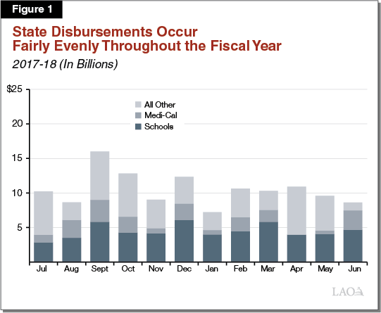
State Makes Disbursements Fairly Evenly Throughout the Fiscal Year. The state disburses money throughout the fiscal year to a variety of entities. For example, the state transfers funds to school and community college districts, makes payments to Medi‑Cal providers, and issues payroll to state employees. Figure 1 shows how these expenditures were disbursed throughout the 2017‑18 fiscal year. As the figure shows, disbursements are mostly even. (In this example, the month of September had notably more disbursements than other months because it was the month the state made a $2.3 billion transfer to the rainy day fund.)

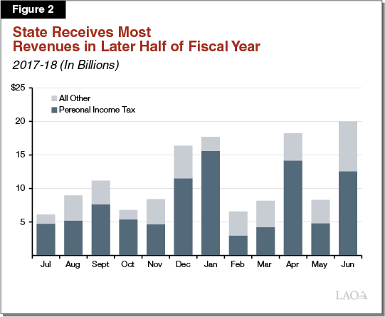
State Receives Most Revenues in Later Half of Fiscal Year. The personal income tax (PIT) is the General Fund’s largest revenue source. As such, the timing of PIT collections has a significant impact on the state’s monthly cash position. Figure 2 shows revenue receipts by month in 2017‑18. As the figure shows, PIT collections are concentrated in four key months: December, January, April, and June. These months correspond with filing deadlines for tax filers who receive large amounts of nonwage income. PIT collections in other months are largely driven by withholding—the amount employers withhold from employees’ monthly paychecks.

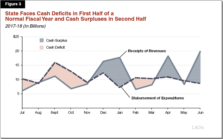
State Faces Cash Surpluses and Deficits Throughout the Fiscal Year. The state’s receipts of revenues and disbursements of expenditures do not perfectly coincide. As such, on any given day during the fiscal year, the state is either receiving more in than it is disbursing (and therefore has a cash surplus) or disbursing more than it is receiving (and has a cash deficit). Cash deficits typically occur early in the fiscal year before the major revenue collection months. Then, later in the fiscal year, particularly in April and June, the state tends to have cash surpluses. Figure 3 shows the cash deficits and surpluses that resulted in the 2017‑18 fiscal year (a year the state had a very healthy budget situation).

Cash Deficits Worsen When Revenues Do Not Meet Expectations. The state’s cash plan for the upcoming fiscal year is based on the total amount of revenue the budget act expects the state will collect. If actual revenues receipts turn out to be lower than anticipated, the state’s cash position will be worse than estimated—with larger cash deficits on a daily and monthly basis.

How the State Controller Manages the State’s Cash Position

The state’s daily cash situation is monitored and managed by the State Controller’s Office (SCO), led by the State Controller, who has the constitutional responsibility to pay the state’s bills.

Routinely Used Cash Management Techniques. The Controller has broad constitutional and statutory powers to manage state cash flows and can use a variety of techniques to address cash flow deficits. As Figure 4 shows, these cash management techniques range from routine to extraordinary. Routinely used techniques include:

• Borrowing From Internal Sources. To manage daily cash deficits, SCO first borrows from internal sources—that is, from state funds other than the General Fund. Some of this borrowing is interest free—for example, borrowing from the Budget Stabilization Account (BSA), the state’s main budget reserve. SCO also can borrow from other internal sources, such as special funds and other funds that are classified as borrowable under law, in many cases with interest. When revenues exceed the General Fund’s cash needs (or if the other fund requires the money for its operations), these funds are repaid. The combined balances of internally borrowable funds varies from month to month. As of June 30, 2019, the state had $57.6 billion in internal borrowable resources to use for cash flow management.
• Borrowing From External Sources. Sometimes internal borrowable resources are insufficient for the General Fund to address its cash deficits. In these cases, the state borrows externally from municipal bond investors. There are two types of external borrowing instruments. First, revenue anticipation notes (or RANs), are usually issued shortly after the budget is passed and mature before the following June. Second, revenue anticipation warrants (or RAWs, but technically called registered reimbursement warrants) can mature after the end of the fiscal year. Unlike RANs, RAWs allow the state to borrow across fiscal years.

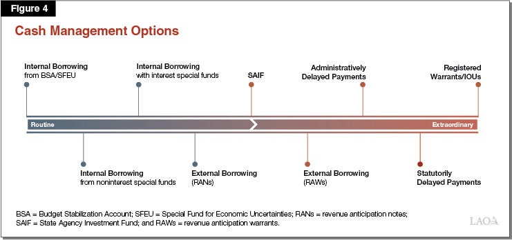
Extraordinary Cash Management Techniques. At certain times, the state faces very serious cash problems and internal and external sources of borrowing are insufficient to address cash deficits. When this occurs, SCO also has some extraordinary measures to use to manage the state’s cash flows. These include:

• Delaying Payments Administratively. State law—as well as contracts and disclosures made to the state’s bond and note investors—establishes that certain state payments should take priority. (Priority payments include, for example, payments to school districts, principal and interest payments on bonds, and employees’ wages and benefits.) Accordingly, when the state’s cash resources are insufficient to meet all budgeted obligations, SCO must make priority payments before making non‑priority payments. In these cases, the Controller can delay non‑priority payments by simply not paying certain bills when they are presented to the office.
• Issuing Registered Warrants (or IOUs). In addition to delaying payments, the Controller has the power to issue registered warrants (also known as IOUs). IOUs allow SCO to delay making payments until they can be redeemed from available General Fund resources. At that point, the recipient can redeem the IOU with interest. In essence, an IOU forces a recipient of state funds (such as a vendor or local government) to provide the state with an involuntary loan.

How the Legislature Has Addressed Cash Deficits

While the executive branch—particularly the Controller—has responsibility for managing the state’s cash position, at various points in state history the Legislature has needed to take action to address the state’s cash issues. In particular, the Legislature has:

• Delayed Payments Statutorily. While the executive branch has some authority to delay payments administratively (as described earlier), some payments can only be delayed with the enactment of statute. For example, in the past, the Legislature has delayed payments to school districts, transfers to local governments, and payments to Medi‑Cal providers.
• Made Some Funds Available for Internal Borrowing. Not all state funds are available for cash flow borrowing. Sometimes these restrictions are constitutional, but in other cases they have been statutory. Over the last decade or so, the Legislature has enacted statutory changes to make billions of dollars from other funds available for cash flow borrowing.
• Created the State Agency Investment Fund. In 2011, the Legislature passed SB 79 (Committee on Budget and Fiscal Review, Chapter 142 of 2011), which created the State Agency Investment Fund (SAIF), a mechanism that allowed the University of California (UC) and California State University (CSU) to lend money to the state for cash flow purposes. The SAIF accepted deposits from the universities and then repaid those funds, with interest, at a later date. Altogether, UC and CSU deposited $2.2 billion into the SAIF in 2011 and 2012, giving the state additional cash resources.
• Authorized Automatic Expenditure Reductions to Facilitate Sales of RAWs. In some cases, the state might not have been able to execute a sale of short term cash instruments in the bond market successfully without a mechanism to give investors more confidence in the state’s ability to repay the debt on time. Consequently, at various points, the Legislature has enacted “trigger legislation” to facilitate the issuance of RAWs. For example, in 1994 the Legislature helped state officials sell a series of RAWs to investors by passing a law that required reductions in most categories of expenditures if cash flow projections showed that timely payment of RAWs was threatened.

How the State Treasurer Invests the State’s Cash

State’s Unused Cash Is Invested in the Pooled Money Investment Account (PMIA). The prior sections described how the Controller pays the state’s bills when the General Fund faces a cash deficit. However, during other months of the year, the General Fund has cash surpluses. These cash surpluses do not sit idle: they are invested by the State Treasurer’s Office in the PMIA. In addition to holding General Fund cash, the PMIA holds the cash of other state funds in the Surplus Money Investment Fund and the cash of some participating cities, counties, and other local entities in the separate Local Agency Investment Fund (LAIF). The PMIA is governed by the Pooled Money Investment Board, which includes the Treasurer, the Controller, and the Director of Finance. The board has a fiduciary duty to safeguard the interests of its investors—the state and local governments with funds invested in the LAIF.

PMIA Investment Earnings Are Relatively Low, but Vary Over Time. By law, PMIA monies can only be invested in certain categories of investments, including: (1) U.S. Government securities; (2) securities of federally sponsored agencies; (3) domestic corporate bonds; (4) interest‑bearing time deposits in California banks, savings and loan associations and credit unions; and (5) prime‑rated commercial paper. The Treasurer typically invests funds in the PMIA in safe instruments with short‑term maturity schedules, meaning the average effective yield of those investments is relatively low—currently around 2.4 percent. However, these average yields have varied substantially over time. In the early 1980s, they were generally above 10 percent, averaged around 6 percent for much of the 1990s, and fell after the dot‑com bust and ensuing recession in the early 2000s. After a brief period above 4 percent in the mid‑2000s, the rate fell nearly to zero after 2008 and remained very low for a number of years. In the last few years the rate has been slowly increasing again.

PMIA Earnings Distributed to General Fund and Other Funds. The entire PMIA pool earns investment returns and then those returns generally are distributed to funds based on their average daily balances (the General Fund is a key exception). For example, for the quarter ending June 30, 2019, the Fish and Game Preservation Fund represented 0.8 percent of the average daily balance of the PMIA and therefore accrued 0.8 percent of its investment earnings for that quarter (in this example, $526,000). After this calculation is conducted for all funds that accrue PMIA earnings on this basis, the remaining quarterly earnings are all distributed to the General Fund. In 2017‑18, the General Fund earned $250 million in PMIA investment revenues.

History of State’s Cash Position

The state’s cash position is currently very healthy, but this has not always been true. This section describes how the state’s cash position has evolved over the last several decades.

Great Depression to 1980s

Cash Management First Becomes Major Issue During the Great Depression. In 1933, the Legislature faced its first cash problem when it anticipated that the General Fund might be exhausted before the end of the 1933‑35 budget biennium. Legislation was enacted to provide that SCO could issue registered warrants when the state was presented with valid claims unable to be paid “for want of funds.” The registered warrants—or IOUs—could bear interest of 5 percent per year. The State Treasurer challenged the constitutionality of the practice. The California Supreme Court upheld the registered warrant law as a valid use of the Legislature’s authority to appropriate state monies and found it did not run afoul of the Constitution’s debt limitation clauses (see box below). A subsequent related case in 1936 challenged the state’s authority to pay registered warrants in the following biennium—that is, to have the liability cross fiscal years. Again, the court found that the Legislature was within its legal authority to do so.

State Issued Its First RANs in the Early 1970s. Facing cash deficits again in the early 1970s, the Legislature enacted a statute that temporarily authorized the Treasurer, in consultation with the Controller, to issue “notes of the State of California representing . . . registered demands” (Chapter 223 Statutes of 1971). Although the statute used different terminology, these notes were equivalent to today’s RANs. The intent of the measure was “to provide the state with additional means of temporary borrowing to meet cash flow needs and avoid more costly registered warrants.” The constitutionality of this new cash management technique was again challenged on the grounds that it violated the Constitution’s debt limitations. Relying on the precedent set in the 1930s cases on registered warrants, the Supreme Court found the use of these notes was allowable. About a month later, the state issued about $500 million in notes under the temporary statute.

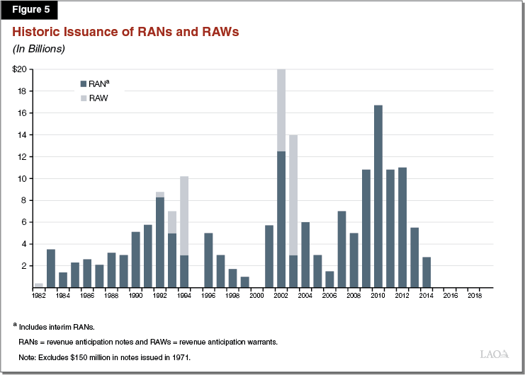
State Began Consistently Issuing RANs in Early 1980s. Over a decade later, in the early 1980s, the Legislature passed a law giving the Treasurer, in consultation with the Controller, permanent authority to issue RANs. As Figure 5 shows, after this point, the state began consistently using RANs to address cash flow deficits—after 1983, California issued RANs every year until 1995. The state also issued its first RAW in 1982, although these instruments were not used again until the state faced a cash crunch a decade later.

Cash Crunches in Early 1990s and 2000s

In the early 1990s and early 2000s, following recessions in each period, the state faced two “cash crunches.” During these periods, the Controller and Legislature both needed to take some extraordinary actions to manage the state’s cash situation.

First Cash Crunch in the Early 1990s. After a recession in the early 1990s, the state faced persistent budget deficits for a number of years. These budget deficits put pressure on the state’s cash position. In 1992, for the first time since the Great Depression, the Controller issued IOUs during a budget impasse. In 1994, the Legislature helped state officials sell a series of RAWs to investors by agreeing in law to automatically reduce most categories of expenditures if cash flow projections showed that timely payment of RAWs was threatened. The early 1990s were marked by a series of sales of RANs and RAWs—at the time, the largest such sales in the state’s history (see Figure 5).

Second Cash Crunch in Early 2000s. After a period of relative calm in the mid‑ and late‑1990s, California faced another series of years with acute budget problems following the dot‑com bust and ensuing recession. Although the dot‑com bust was relatively mild in economic terms, it hit the California budget—which is particularly reliant on the Bay Area’s technology sector—especially hard. Again, budgetary problems put pressure on the state’s cash position as revenue receipts came in lower than expected. In these years, the state issued historically large RANs and RAWs—with total short‑term borrowing of $20 billion issued in 2002 alone.

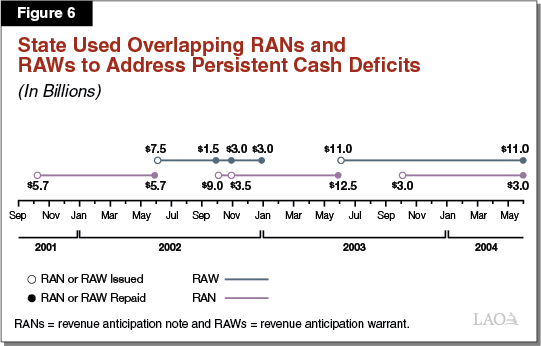
State Used Overlapping RANs and RAWs to Address Persistent Cash Deficits in Early 2000s. RANs and RAWs are short‑term cash instruments—even the longer‑term RAWs usually mature about a year after issuance. However, with the state facing persistent cash deficits in the early 2000s, these instruments took on a longer‑term quality because new debt was issued to replace maturing debt from previous sales. Figure 6 shows how this worked—with each sale of a new RAN replacing a maturing RAW and vice versa. This means that continuously from October 2001 to June 2004 the state had billions of dollars in outstanding cash deficit financing.

Cycle Ends With Authorization of Economic Recovery Bonds (ERBs). The cycle of overlapping RANs and RAWs ended in 2004 when voters authorized $15 billion in long‑term bonds, known as ERBs, to pay off the state’s accumulated budget deficits. (The same measure also prohibits the state from using this tool again in the future.) In the 2004‑05 fiscal year, the state issued roughly $11 billion in ERBs—leaving the remainder for future issuance. ERBs were a tool to address a budget deficit, not a cash deficit. Nonetheless, issuing ERBs allowed the state to address budgetary deficits in the short term and, by giving the state additional cash, meant the state no longer needed to issue the same quantity of cash flow borrowing.

Cash Crisis in 2008‑09

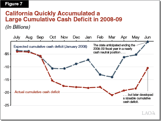
Early in the Great Recession, the State Could Not Anticipate the Depths of Its Cash Deficits. In January 2008 the state had just entered the Great Recession, but policymakers had little knowledge of how deep the recession would be, nor the extent of its impact on the state’s financial situation. Figure 7 compares the state’s expected cumulative cash deficits for each month of 2008‑09 to its actual cash deficit (measured in January 2010). As the figure shows, in January 2008, well before the fiscal year had started, the administration expected the state would end the fiscal year with a cumulative cash deficit close to zero—meaning the state would disburse roughly what it had received in revenues. However, what actually happened was quite different. Revenues in this year came in far below expectations, meaning the cash deficit went below $20 billion and the year ended with a cumulative cash deficit of $10 billion.

California Faced a Frozen Credit Market in September of 2008. Near the end of 2008, the state understood the extent of its cash needs, but found itself unable to address those needs with external borrowing. The Legislature passed the 2008‑09 Budget Act on September 15, 2008—the same day Lehman Brothers filed for bankruptcy. In the following weeks, California approached the bond market for cash flow borrowing and found the U.S. credit market had frozen, partly in response to the financial market uncertainty accentuated by Lehman Brothers’ collapse. On October 3, 2008, Governor Schwarzenegger wrote to the Secretary of the U.S. Treasury alerting him to the possibility that California might ask the federal government for short‑term financing—an unprecedented move for the state.

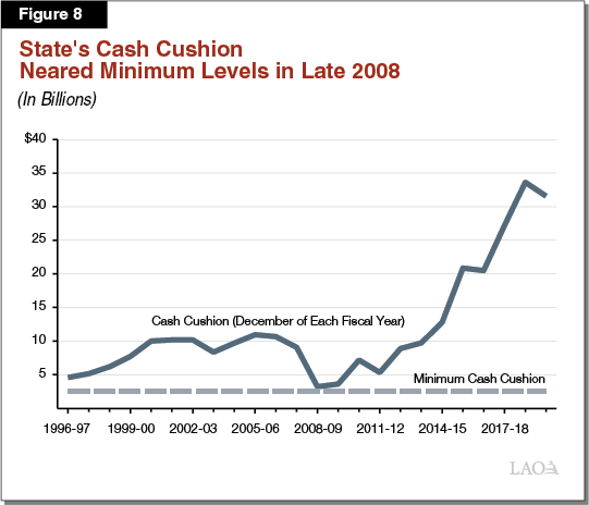
The State Depleted Its Internal Borrowable Resources by the End of 2008. As a result of falling state revenues and the state’s inability to access sufficient external borrowing, around the end of 2008, the state neared its minimum “cash cushion.” This minimum cash cushion is the dollar amount of internal borrowable resources that are left unused—or the daily amount that are not being used to meet the state’s disbursements. In these years, SCO had set a minimum cash cushion of $2.5 billion for the end of each month (although cash levels within the month fluctuated below that level). Figure 8 shows the state’s cash cushion in December of each fiscal year from 1996‑97 to 2018‑19 (a month when the state often reaches its annual cash balance lows). The figure displays month‑end cash, so the state reached even lower levels in some of these years within the month. As the figure shows, the state’s cash cushion dropped substantially between 2007‑08 and 2008‑09, and in December 2008 nearly fell below the minimum level.

Throughout the Crisis, the Controller Took Many Extraordinary Actions. The state did not ultimately request aid from the federal government for cash deficit financing. Instead, throughout the Great Recession, the Controller and Legislature took a number of extraordinary actions to address the state’s cash flow shortfalls. This included delaying billions of dollars in payments and the Controller issuing billions of dollars in IOUs. At this time, in the midst of the state’s budgetary crisis, the Governor also made an unprecedented proposal to use a cash flow borrowing instrument to finance the state’s budget deficit. This proposal, although never adopted, is described in more detail in the box below.

Cash Crisis Was Unique Because of External Constraints. Before 2008, the state had faced significant cash deficits as a result of weak revenues. The state also had issued large, short‑term bonds previously. The cash crisis in 2008‑09 was unique not because the state needed to borrow significant amounts from external sources but because the state found itself unable to do so. For a number of days in October of 2009 the state confronted a very real possibility that it would not be able to issue a RAN large enough to meet its cash obligations. As a state government, California has the power to levy taxes and cannot declare bankruptcy. These factors make the state a reliable borrower. Nonetheless, the state cannot access a credit market that is either unwilling or unable to lend to it.

Today: A Dramatic Improvement in California’s Cash Situation

The state’s cash situation today is dramatically different. As Figure 5 above showed, after decades of issuing RANs nearly every year, the state has not issued a RAN since 2014. Instead, the state has exclusively used internal borrowable resources to manage its cash situation.

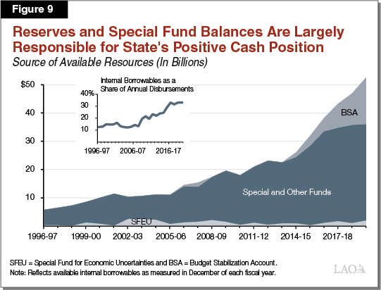
State’s Internal Borrowable Resources Are at a Historic High . . . A key reason that the state has not needed to issue a RAN for years is that internal borrowable resources have reached a historic high, both in dollar terms and as a share of disbursements. At the end of 2019‑20, SCO estimates the state will have $54 billion in internal borrowable resources available, representing about one‑third of that year’s total disbursements. As the top part of Figure 9 shows, this level of internal borrowable resources as a share of disbursements is higher than at any other point in the last several decades.

. . . Primarily Due to Increased Reserves and Other Fund Balances. The largest single contributor to these sizable balances are the state’s budgetary reserves, most notably the BSA. Since 2014, largely as a result of strong revenue growth and legislative choices, the state has been making sizable annual deposits into the BSA. By the end of 2019‑20, the fund is expected to reach $16.5 billion and currently represents 28 percent of the state’s total internal borrowable resources. The second reason the state’s internal borrowable resources have increased is that balances in special funds and other funds—such as nongovernmental cost funds—also have increased. These increasing balances are shown in dark blue in Figure 9.

Other Fund Balances Have Increased for a Few Reasons. There are a few reasons that the cash balances in special funds and other funds have increased substantially, particularly over the last decade. They are:

• Legislature Has Made Some Existing Funds Borrowable. As was discussed earlier, the Legislature has passed laws to make a number of funds borrowable that in the past were not. For example, the February 2009 budget package for the 2009‑10 budget made about $3 billion in special funds borrowable for cash flow purposes.
• State Has Created Some New Funds. The state has created some new funds that have substantial balances and are now available for cash flow borrowing. For example, in 2012 the Legislature created the Greenhouse Gas Reduction Fund (GGRF), which receives revenues from the state’s cap‑and‑trade program. On a cash basis, the fund now stands at $7.7 billion (as of June 30, 2019)—representing over 13 percent of the state’s internal borrowable resources. (The Department of Finance’s [DOF’s] most recent estimate of the budgetary balance of GGRF is much lower—$1.3 billion for the end of 2018‑19. The box below describes why funds’ balances differ on a budgetary versus cash basis.)
• Balances in Some Existing Funds Have Grown. Finally, balances in some existing funds have increased over time. For example, the Unemployment Compensation Disability Fund collects revenues from a state payroll tax and finances short‑term disability insurance and paid family leave. On a budgetary basis, this fund has grown from several hundreds of millions of dollars in the early 2000s to over $3 billion in 2019. On a cash basis, the fund had $3.5 billion on June 30, 2019—which represents 6 percent of total borrowable resources. In this example and others, balances in existing funds have grown as revenues to those funds also have grown.

Recent Borrowing from State’s Cash Pool

Reflecting the state’s positive cash situation, the balance of the state’s cash pool—the PMIA—has increased in recent years. The average daily balance of the PMIA was $97.7 billion for the second quarter of 2019, although it was $74.1 billion excluding local governments’ funds. The balance of the PMIA has also grown remarkably in recent years. In fact, from 2015‑16 to the end of 2018‑19 the PMIA grew by about $30 billion.

With this increased liquidity, the state has had the capacity not only to cover its internal cash flow needs, but also to use the state’s portion of the cash pool to make loans. Twice in the last few years, the Legislature has authorized the executive branch to borrow from the state’s cash resources and allocate the funds to specified uses. In this section, we describe these two recent legislative actions and how they have affected the state’s cash position.

Senate Bill 84

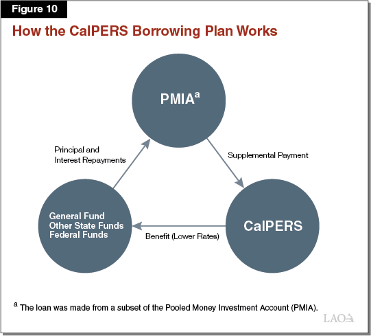
As part of the 2017‑18 budget package, Chapter 50 of 2017 (SB 84, Committee on Budget and Fiscal Review) approved the Governor’s May Revision proposal to borrow $6 billion from a portion of the PMIA to make a one‑time supplemental payment to the California Public Employees’ Retirement System (CalPERS). Figure 10 shows how this borrowing plan is meant to work. Under the plan, the Controller has transferred $6 billion from the PMIA to CalPERS, which CalPERS has invested to help pay down its unfunded liability, earning an expected return of 7 percent per year. Over the next few decades, funds that pay pension costs accrue benefits through lower employer contributions costs relative to what they would be otherwise. Finally, funds that accrue these benefits are to repay the loan to the PMIA with interest.

Repaying the Loan. Under the CalPERS borrowing plan, the General Fund eventually will repay about 50 percent of the loan and other funds will repay the remaining 50 percent. The General Fund’s share of the loan will be repaid from the state’s annual Proposition 2 (2014) debt payment requirements. (These requirements vary from year to year according to a formula, but are generally $1 billion or more depending on expected state revenue performance.) Other funds are to repay their shares using their own available resources. As a result, in the case of the General Fund’s share of the loan, the state has a well‑defined plan for the stream of repayments.

Effect of SB 84 on State’s Cash Balances. Senate Bill 84 initially affected the state’s cash position by lowering internal borrowable resources by $6 billion relative to what they would have been otherwise. As this loan is repaid with interest, internal borrowable resources will increase again. By the end of 2019‑20, the state will have repaid nearly $2 billion of this loan (including interest, the state likely will make around $7 billion in total repayments). The outstanding amount of SB 84 borrowing is not particularly large in the context of the state’s overall internal borrowable resources. That said, the duration of this loan could be relatively long. Statute requires the loan to be repaid by 2030, meaning it could result in lower cash balances for over a decade.

Assembly Bill 1054

Chapter 79 of 2019 (AB 1054, Holden) created a fund to help cover the costs of investor‑owned utilities’ liabilities for wildfire claims when those utilities are legally liable. The law requires the utilities to meet certain conditions to participate, including contributing at least half of the fund balance with shareholder contributions. Should the utilities meet those conditions, the law will allow them to access funds that they can use to pay out wildfire liability claims. (The two currently eligible investor‑owned utilities have stated they intend to participate. Pacific Gas and Electric [PG&E] is not eligible to participate until it has exited bankruptcy protection.) The law scheduled an initial loan of $2 billion from the state’s portion of the PMIA to establish the fund and, potentially, pay initial claims. The law also gives the Director of Finance the authority to make an additional loan of up to $8.5 billion to provide more initial capitalization for the fund.

Repaying the Loans. In the new law, the Legislature has stated its intent to repay the loan from the state’s cash resources as quickly as possible. To accomplish this, the law authorizes the state to issue bonds to repay the loan with interest. The debt service on those bonds will be repaid with revenue from a surcharge on ratepayers’ bills. This surcharge will replace an existing one that is currently funding the debt service on a different set of Department of Water Resources (DWR) bonds, which are expected to be fully repaid near the end of 2020. Once those existing DWR bonds are fully repaid, the new bonds—to backfill the state’s cash resources—can be issued.

Effect of AB 1054 on State’s Cash Balances. Similar to SB 84, AB 1054 affects the state’s cash position by lowering internal borrowable resources relative to what they would have been otherwise. The total amount authorized is large, although the initial loan of $2 billion is relatively small in the context of the state’s overall internal borrowable resources. The overall effect of AB 1054 on the state’s cash balances is yet to be seen—it will depend on decisions by the administration about how much to transfer to the fund, when to make those transfers, and when to issue the new bonds to repay the loan. (These decisions will depend in part on whether PG&E participates or not.) Depending on these decisions, the effect on the state’s cash balances could be relatively significant or not.

What Will Happen in the Next Recession?

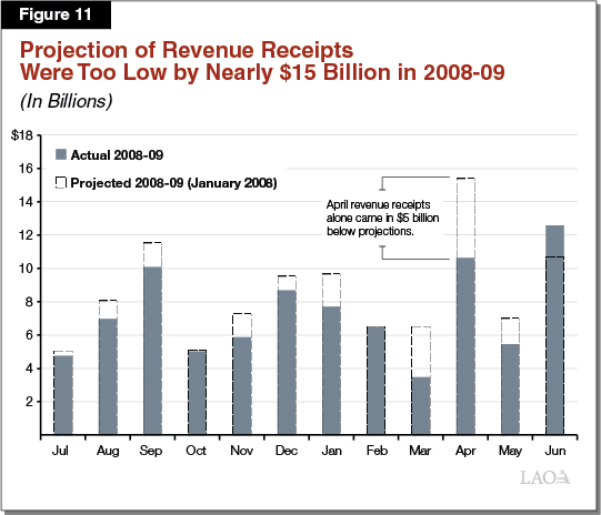
Revenue Receipts Will Be Lower Than Anticipated. When the Legislature passes a budget for an upcoming fiscal year, it does not know if a recession will occur or, sometimes, if one already has started. When a recession occurs, revenues come in lower than both budget and cash projections anticipated, resulting in lower receipts. This is precisely what occurred, for example, in the 2008‑09 budget. When DOF prepared the cash projections for 2008‑09 in January 2008, policymakers might have understood budgetary problems were emerging, but did not know how deep the revenue drops would be. As Figure 11 shows, the projections of revenue receipts for 2008‑09 were too low by nearly $15 billion, with receipts from April alone off by $5 billion. In the next recession, estimates of revenue receipts will again be too high and cash deficits—and the state’s borrowing needs—will increase.

Balances of Internal Borrowable Resources Will Decline. In the next recession, the balance of internal borrowable resources likely will decline relative to their current levels. There are two primary reasons for this:

• Budget Reserve Balances Will Decline. When revenues do not meet expectations, a budget problem usually emerges. For the first time in the state’s recent history, the Legislature will have a significant reserve available (in the BSA) to address a budget problem in the next recession. While these resources are currently available for cash management, once they are appropriated and eventually disbursed, they will no longer be available for this purpose.
• Other Internal Borrowable Sources Will Decline. In addition to declines in the BSA, in the next recession, the balances of other borrowable sources also likely will decline. There are two reasons for this. First, the Legislature might address a future budget problem by borrowing from special funds. Budgetary borrowing from a special fund that also is available for cash flow borrowing does not initially change the total amount available for borrowing, but it does eventually once the funds are disbursed. Second, the cash balances in some special funds could decline for other reasons, for example, because of their own revenue declines or expenditure increases.

State Could Need External Borrowing. In a future recession, when cash deficits become larger and internal borrowable resources decline, the state might require external borrowing to address cash flow deficits. Although there are advantages to primarily relying on internal borrowable sources for cash management, issuing short‑term debt to meet cash management needs is not inherently problematic. Such borrowing is historically a routine part of the state’s cash flow management and it carries relatively low interest rate costs.

Key Takeaways

The State’s Cash Position Is Now Very Strong

After a long history of cash problems over several decades, the state’s cash position is now very good. After decades of issuing RANs nearly every year, the state has not issued a RAN since 2014. Instead, the state exclusively has used its sizable internal borrowable resources to manage its cash situation. This positive situation is the result of a number of factors, including: strong revenue growth, the state building a sizable budget reserve, and the growing balances of other funds. In fact, the state’s cash situation is so positive that the Legislature has been able to commit a small part of this liquidity pool to make loans to fund other priorities—including reducing the state’s long‑term pension debt and creating a fund to address utilities’ liabilities arising from wildfire claims.

The State Likely Will Have Time to Anticipate a Problem. A key advantage of having a high amount of internal borrowable resources before the next recession is that although those resources will decline, they are unlikely to decline very rapidly. In short, having this significant cushion buys the Legislature time and likely will allow the state—including the Controller and Treasurer—to anticipate a cash problem in advance. Those entities will then have time to take corrective actions before a crisis occurs.

The State’s Cash Position Will Not Always Be This Strong

In the next recession, the state’s cash position will decline. Revenue receipts will be lower than anticipated, creating larger cash deficits, and the balances of internal borrowable resources will decline as the state uses its rainy day fund to cover budget deficits. For example, using $10 billion from the BSA to cover a budget deficit would mean the state’s internal borrowable resources are lower by $10 billion by the end of the fiscal year. These risks also are correlated—when one condition deteriorates (for example, revenues failing to meet expectations) other conditions also likely will deteriorate.

A key lesson from the cash crisis of 2009 is that the state’s cash situation is not only a matter of internal choices but also of external factors beyond the state’s control. When internal resources are insufficient, the state relies on the external bond market to finance its monthly cash deficits. That market might, at times, be unable or unwilling to lend to California. Although the series of events at the end of 2009 represented a true crisis, the factors that led to it were relatively unique. The chances that the state will face a problem precisely along those lines again in the future are low. Nonetheless, the state likely will face some kind of cash challenge again in the future.

A Framework to Evaluate Future Cash Loans

The Legislature has authorized two loans from the state’s cash resources in the past few years. While we are not aware of any plans for a future loan, given the high level of internal borrowable resources, a future proposal is possible. Neither of the existing loans has yet compromised the state’s internal liquidity. However a future loan, coupled with these existing ones, has the potential to jeopardize the state’s cash position in the next recession. To help the Legislature evaluate the risk of a future proposed loan, this section outlines some criteria that the Legislature might want to consider.

Size of the Loan. The first consideration in evaluating the risk of a future loan is its size: in particular, the size of the loan relative to the amount of internal borrowable resources likely to be available in the next recession. A loan of only $1 billion represents a small portion of the state’s cash cushion and is unlikely to substantively affect the state’s cash management needs. A loan of $10 billion would be more noticeable in the state’s cash position, particularly when internal borrowable resources decline by billions of dollars.

Duration of the Loan. In the case of a large proposed loan, its duration becomes an important consideration. That is because these loans become more significant problems if they are still outstanding when the next recession occurs. As such, the longer the duration of a cash pool loan, the more risky it is. This means there are two key considerations for the Legislature in evaluating a future loan: (1) its duration and (2) the timing of the next recession. Of course, no one can know when the next recession will occur. Nonetheless, in evaluating a future loan, the Legislature must make a judgment about the likelihood that a recession will occur while the loan is still outstanding.

Dependability of Repayments. Another key consideration for the Legislature in making future cash loans is the degree of certainty with which the loan will be repaid. Loans made with a dedicated revenue or resource stream—such as SB 84—are more likely to be repaid promptly than loans repaid using all‑purpose General Fund resources.

Fiscal Benefit. In evaluating any future cash loan, we would finally encourage the Legislature to consider the loan’s potential fiscal benefit using high‑quality, rigorous quantitative analysis. Loans that result in substantial fiscal benefit to the state are more advantageous than those that do not. One key benefit of SB 84, for example, is that it likely will have a substantial fiscal benefit to the state—the loan is likely to result in billions of dollars in savings to the state over time.

Conclusion

After nearly two decades of persistent budgetary problems and a fluctuating cash position, California is now enjoying both healthy budget and cash situations. As with the state’s budget situation, this positive cash position is unlikely to last forever. When a recession occurs, it will mean lower revenue receipts, larger cash deficits, and declining balances of internal borrowable resources. Moreover, these risks are correlated—when one condition deteriorates (for example, revenues failing to meet expectations) other conditions also are likely to deteriorate. Given this, the Legislature will want to consider any additional loans from the state’s cash resources carefully. In particular, assessing the size, duration, security, and benefit of the loan can help the Legislature determine whether the reduction in borrowable resources is merited.