LAO Contacts

January 6, 2020
Assessing California's Climate Policies—Electricity Generation
- Introduction
- Overview of Electricity Sector Emissions
- LAO Assessment of Policies
- Key Issues for Legislative Consideration
- Conclusion
- Appendix
Executive Summary
Chapter 135 of 2017 (AB 398, E. Garcia) requires our office to report annually on the economic impacts and benefits of the state’s greenhouse gas (GHG) limits. In this report, we assess the effects of some of the state’s major policies intended to reduce GHG emissions from the generation of electricity.
Electricity Sector Primary Driver of GHG Emission Reductions. Over the last decade, the electricity sector has been the primary driver of statewide GHG emission reductions. Annual emissions from the electricity sector have declined by about 40 million metric tons (40 percent) over this period. Reductions have mostly been due to a change in the mix of resources used to generate electricity—primarily large increases in renewables (solar and wind) and, to a lesser extent, reductions in the amount of coal.
State Policies Likely Key Factors in Reductions, but Magnitude of Effects Uncertain. In total, state policies were likely substantial drivers of changes to the generation mix that lowered annual emissions. However, a wide variety of other factors likely influenced emissions over the same period, including declines in natural gas prices, declines in prices for renewable generation, and federal policies. We did not identify any academic studies that comprehensively evaluated the overall effects attributed to state GHG reduction policies.
RPS Likely a Substantial Driver of Emission Reductions at Moderate Cost Per Ton. Based on some “back‑of‑the‑envelope” calculations, we estimate that the Renewable Portfolio Standard (RPS) program (1) reduced annual emissions by up to the low tens of millions of tons in 2018 and (2) costs about $60 to $70 per ton reduced in energy procurement costs. A variety of other costs—such as transmission and integration costs—are difficult to quantify, but could increase costs by tens of dollars per ton. Although the program likely generated other benefits—such as reducing local air pollutants and contributing to a global decline in solar prices—the magnitude of these effects appears to have been relatively small. Importantly, future costs to increase renewable generation are likely to be much different than past costs. This is because procurement costs for renewable energy are likely to be much lower in the future due to declining renewable prices, but this could be at least partially offset by higher integration costs.
Rooftop Solar Policies Generally More Costly. State policies—such as the California Solar Initiative (CSI) and net energy metering (NEM)—likely had a significant impact on the amount of electricity generated from rooftop solar, which has reduced annual emissions by several million tons. However, these policies generally were a more expensive method for reducing emissions than policies focused on utility‑scale renewables. Costs of electricity from distributed solar are at least a couple of times higher than utility‑scale solar. Furthermore, estimated costs of emission reductions under CSI were about $150 to $200 per ton. The overall effects of NEM are not clear, but the policy has likely resulted in a substantial financial cost‑shift from solar customers to nonsolar customers. The magnitude of other potential advantages of rooftop solar—including knowledge “spillovers” from learning‑by‑doing and reduced distribution system costs—are less clear, but appear to be relatively small.
Little Known About Effects of SB 1368 and Cap‑and‑Trade on Emissions. Although a 2006 state law that prohibited new long‑term contracts with coal power plants (Chapter 598, SB 1368 [Perata]) likely reduced emissions from coal generation, we did not identify any empirical research assessing the magnitude of the effects. For cap‑and‑trade, the level of costs is clearer than the level of emission reductions. Market prices for allowances suggest the marginal costs for emission reductions encouraged by the program have been less than $20 per ton, but the overall amount of emission reductions from electricity generation attributable to the program are unclear. The cap‑and‑trade program has had significant distributional effects in the electricity sector. Specifically, the overall financial benefit to residential electricity customers from utilities selling allowances and using the proceeds to benefit ratepayers has exceeded the compliance costs that have been passed on to customers.
Resource Shuffling Potentially Offsets Some of the Emission Reductions. Resource shuffling occurs when the mix of existing electricity supplies changes so that more low‑carbon electricity is sent to California while more high‑carbon electricity is sent to other states. Several different prospective analyses showed that there was potential for significant resource shuffling from imports. There has been limited retrospective empirical research estimating resource shuffling, but some preliminary work suggests it could be a significant factor.
Key Issues for Legislative Consideration. We identify some key issues for the Legislature to consider as it modifies and adopts policies to achieve its GHG goals.
- Comprehensive Policy Evaluations Lacking. Although the amount of information varies by program, we found a lack of rigorous retrospective evaluations for some programs and effects. The Legislature might want to consider directing agencies to identify opportunities to facilitate retrospective evaluation by ensuring data is available to researchers and, potentially, designing programs in ways that allow for more robust evaluations. In addition, the Legislature could consider additional reporting requirements and/or funding for research efforts in key areas, including resource shuffling and the effect of distributed solar on distribution system costs.
- Mix of Policies Likely Not Most Cost‑Effective Way to Reduce GHGs. There has been substantial differences in the costs of reducing emissions between cap‑and‑trade (marginal cost that are currently less than $20 per ton), RPS (average costs of about $60 to $70 per ton or more), and policies promoting distributed solar (average costs of roughly $150 to $200 per ton). In the future, the Legislature might want to rely more heavily on the most cost‑effective programs, such as cap‑and‑trade. In certain limited instances, the Legislature could consider adopting policies that are a somewhat more costly way to reduce GHGs if those policies result in substantial benefits in other ways, such as reducing local air pollution and creating knowledge spillovers.
- High Electricity Prices Could Be a Barrier to GHG Reductions. Retail electricity rates are substantially higher than the marginal social costs of providing electricity. This is due to a variety of factors including (1) utilities recovering fixed costs through volumetric rates, (2) declining electricity consumption (which means fixed costs are spread over a smaller base), and (3) costs for various state‑mandated programs. High electricity rates discourage adoption of some technologies—such as electric vehicles and electric appliances—that could be used to substantially reduce statewide GHGs. As a result, the Legislature might want to consider actions that more closely align retail electricity rates with the marginal costs of providing the electricity. For example, the Legislature could direct regulators to exclude at least some of the fixed costs and certain state policy costs from utilities volumetric electricity rates, and potentially fund them in other ways.
Introduction
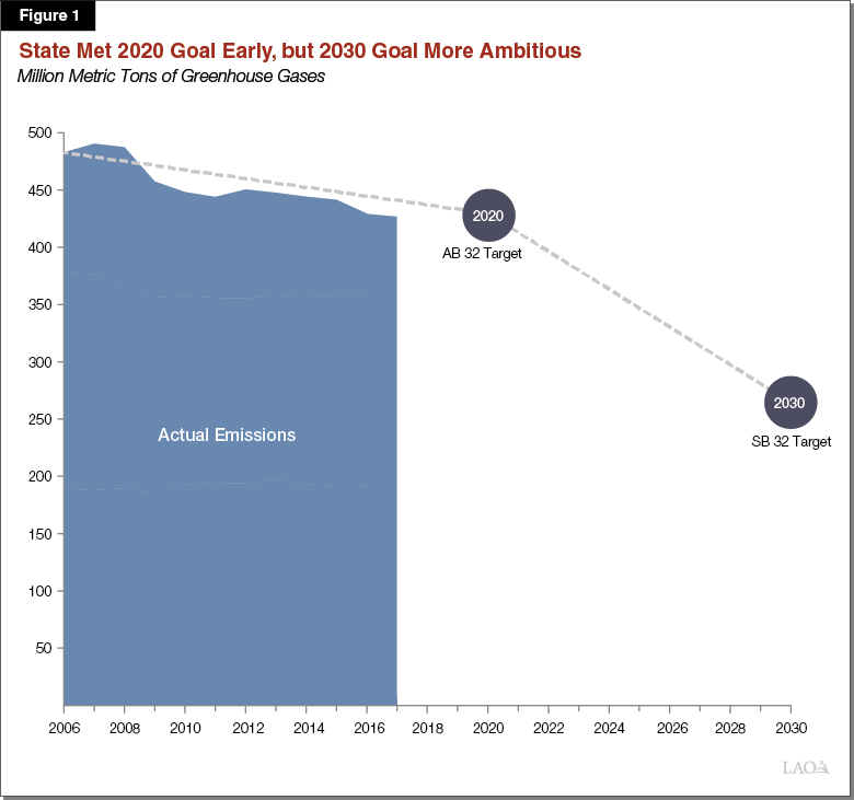
Chapter 488 of 2006 (AB 32, Núñez/Pavley) established the goal of limiting greenhouse gas (GHG) emissions statewide to 1990 levels—431 million metric tons (MMT) of carbon dioxide equivalent (CO2e)—by 2020. In 2016, Chapter 249 (SB 32, Pavley) extended the limit to 40 percent below 1990 levels—259 MMT of CO2e—by 2030. As shown in Figure 1, emissions have decreased since AB 32 was enacted and were already below the 2020 target in 2017. However, the rate of reductions needed to reach the SB 32 target are much greater.
Chapter 135 of 2017 (AB 398, E. Garcia) requires our office to report annually on the economic impacts and benefits of the state’s GHG limits. In 2018, we issued two reports in fulfillment of this requirement. First, we released Assessing California’s Climate Policies—An Overview, which provided the analytical framework we are using to assess the economic impacts and benefits of climate policies. Second, we released Assessing California’s Climate Policies—Transportation, which applied that framework to the various state programs designed to reduce GHG emissions from the transportation sector. In this report, we assess the effects of the state’s major policies intended to reduce emissions from the generation of electricity—hereafter referred to as electricity generation or electricity supply. (We do not assess the effects of programs primarily intended to reduce electricity consumption, such as energy efficiency programs, in this report.)
Overview of Electricity Sector Emissions
Electricity Sector Background
Overview of Electric Grid. A wide variety of entities—both public and private—play a role in providing electricity to California households and businesses. In general, there are three main parts of the electric grid:
- Generation. Electricity frequently is generated at large power plants (such as natural gas, coal, or nuclear power plants) or large renewable generation sites (such as wind farms or solar fields). This large‑scale generation is also known as utility‑scale generation. These power plants typically are owned by private companies (including some utilities). Some generation occurs at a smaller scale, such as solar installed at residences, businesses, or other smaller‑scale community locations. This smaller‑scale generation is known as distributed generation and usually is owned by the property owner or a third‑party company that installs and owns the generation source.
- Transmission. Electricity generated at utility‑scale is transported through high‑voltage power lines known as transmission lines. These lines typically are owned by utilities. In some cases, electricity is sent directly from transmission lines to end customers, such as large manufacturing facilities.
- Distribution. Generally, electricity is transferred from high‑voltage transmission lines to low‑voltage distribution lines before it is delivered to customers. For example, distribution lines are often on wooden poles that run through cities and neighborhoods. Utilities—both public and private—own and operate distribution lines.
Load Serving Entities (LSEs) Procure Electricity and Deliver it to Customers. Load serving entities provide electricity to end users. They are responsible for generating or purchasing electricity and ensuring it is delivered to households and businesses. Historically, investor‑owned utilities (IOUs) and publicly owned utilities (POUs) have been the primary LSEs. IOUs are private companies regulated by the California Public Utilities Commission (CPUC). POUs are public agencies governed by locally elected or appointed officials. More recently, other types of nonutility LSEs are providing an increasing share of electricity to customers. These include community choice aggregators (CCAs), which are local government‑run entities that buy electricity for customers but use IOU distribution to deliver the electricity, and electric service providers (ESPs), which are private entities that sell electricity directly to commercial customers in IOU territories. In 2018, IOUs provided about 55 percent of electricity to California customers, POUs provided about 25 percent, and CCAs and ESPs provided about 10 percent each.
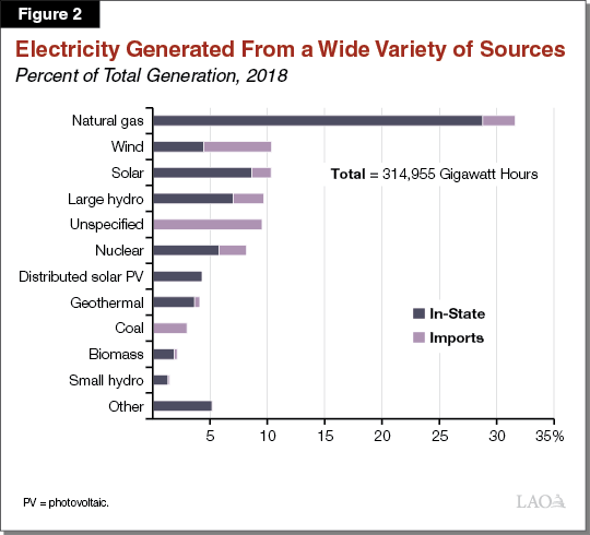
Electricity Generated From a Wide Variety of Sources. Figure 2 shows the different generation sources used to generate electricity that is consumed in California. Natural gas is by far the largest source of generation. Wind, solar, large hydroelectric, unspecified imports, and nuclear contribute a significant share as well. (Unspecified imports are imported electricity where it is not possible to identify the specific generation sources used to produce the electricity.) Roughly 70 percent of electricity consumed in California is generated in‑state and the remaining 30 percent is generated out of state but imported into California through transmission lines.
Major Policies to Reduce Electricity Sector Emissions
The electricity sector accounts for 16 percent of statewide GHG emissions, according to the California Air Resources Board (CARB) statewide GHG inventory. In addition to the statewide GHG goals discussed above, in recent years the state has established GHG goals that are specific to the electricity sector. This includes Chapter 547 of 2015 (SB 350, de León), which requires CARB to establish 2030 GHG targets for the electricity sector (set at a range of 30 MMT to 53 MMT). In addition, Chapter 312 of 2018 (SB 100, de León) establishes a state policy of 100 percent zero carbon electricity by 2045. Over the past couple of decades, the state has implemented a variety of policies intended to reduce GHG emissions from electricity generation. Figure 3, summarizes some of the major policies, which we describe in more detail below.
Figure 3
Summary of Major Policies to Reduce Emissions From Electricity Generation
|
Policy |
Year Implemented |
Description |
|
Renewable Portfolio Standard |
2003 |
Requires LSEs to generate a minimum percent of retail electricity from qualifying renewable sources. Percentages increase over time from 20 percent in 2010 to 60 percent in 2030. |
|
California Solar Initiative |
2007 |
Provided $2.7 billion over a ten‑year period for financial incentives to reduce the cost of installing distributed solar, such as rooftop solar PV. |
|
Net Energy Metering |
1996 |
Encourages customers to install distributed solar generation by paying them a retail electricity rate for the electricity they generate. |
|
Emissions Performance Standard (SB 1368)a |
2007 |
Effectively prohibits LSEs from signing or extending long‑term contracts with coal power plants. |
|
Cap‑and‑trade |
2013 |
Requires electricity generators and importers to obtain an allowance or offset to cover each ton of GHG emitted. Program includes other emitters outside of the electricity sector, and entities can buy and sell allowances. |
|
aChapter 598 of 2006 (SB 1368, Perata). LSE = load serving entity; PV = photovoltaic; and GHG = greenhouse gas. |
||
Renewable Portfolio Standard (RPS). State law requires LSEs (with a few exceptions) to provide a minimum percent of retail electricity sales from qualifying renewable generation. Qualifying renewables include solar, wind, biomass, geothermal, and small hydroelectric. Notably, under current law, some generation sources that do not directly emit GHGs, such as large hydroelectric and nuclear, do not qualify under RPS. Distributed generation, such as rooftop solar PV (photovoltaic), technically can qualify. However, in practice, very little of it is used to comply in part because certain administrative actions needed to certify RPS eligibility can be expensive for smaller PV units.
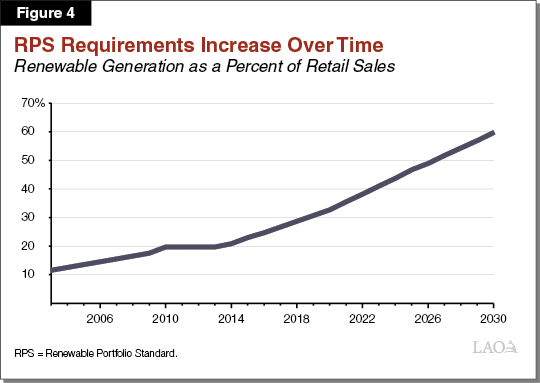
The Legislature has increased or extended the RPS requirements a few different times over the last couple of decades. Chapter 516 of 2002 (SB 1078, Sher) established a 20 percent RPS by 2017, and Chapter 464 of 2006 (SB 107, Simitian) accelerated the 20 percent requirement to 2010. Subsequently, Chapter 1 of 2011 (SBX1 2, Simitian) established a 33 percent requirement by 2020. In 2015, SB 350 established a 50 percent requirement by 2030—a target that SB 100 increased to 60 percent a few years later. State law and regulations also establish interim RPS requirements and targets. Figure 4, shows the RPS requirements under current law and regulation.
The CPUC oversees IOU, CCA, and ESP compliance. The California Energy Commission (CEC) oversees POU compliance. An LSE complies by “retiring” enough renewable energy credits (RECs) to cover its required RPS percentage of retail sales. A REC is a certificate demonstrating that one unit of electricity was generated and delivered from an eligible renewable resource. State law establishes other requirements about what types of RECs may be used to comply (such as a maximum percent of RECs from renewable energy that was generated in other states, but not delivered to California).
California Solar Initiative (CSI). In 2006, Chapter 132 of 2006 (SB 1, Murray) provided state agencies the authority to establish several programs aimed at providing incentives for distributed solar—an effort known as Go Solar California. The overall goal was to install 3,000 megawatts of distributed solar and transition the solar industry to a point where it could be self‑sustaining. The biggest program used to achieve this goal was the CSI, which provided financial incentives to install rooftop solar on businesses and existing homes in IOU territories. Other programs included the New Solar Home Partnership Program, which provided financial incentives for solar on newly constructed homes, and a wide variety of solar programs offered through POUs. The statewide budget for these programs was $3.3 billion over a ten year period—from 2006 to 2016—with about $2.7 billion going to the CSI. The programs were primarily funded through a surcharge on electricity bills.
The CSI included several different subprograms that provided customer incentives for distributed solar. The largest subprogram—called the General Market Program—provided a total of about $2 billion in upfront financial incentives (primarily rebates—based on per kilowatt of generation capacity—to offset the upfront cost of the solar unit) for businesses and existing homes installing rooftop solar. The program had a declining incentives structure. The incentives started high and then automatically decreased over time as each IOU hit certain thresholds for the total amount of solar installed in its jurisdiction. The incentives reduced the cost of installing a residential solar unit by about 25 percent in the early years of the program and by about 5 percent to 10 percent in the final years. This design was intended to gradually reduce customer reliance on subsidies as the solar industry matured and market prices declined. The General Market Program stopped accepting applications for incentives in 2016.
Net Energy Metering (NEM). The vast majority of rooftop solar customers are enrolled in NEM, which supports onsite solar installations. Some version of NEM has been in place since 1996, but has been modified several times since then. Under NEM, the utility effectively pays solar customers (through a bill credit) for the excess electricity they generate that is exported back to the grid. Under NEM, the customer receives the retail rate for electricity, which includes costs associated with generation, transmission, and distribution. For example, if a customer consumes 100 kwh of electricity from the grid, but exports 70 kilowatt hours of electricity from their solar panels back to the grid, then the customer would pay the retail rate for 30 kwh of electricity. In response to state legislation, CPUC made some changes to the NEM program in 2016. Much of the basic structure described above remains in place. Some of the key changes included charging new NEM customers a one‑time interconnection fee and a requirement that new NEM residential customers use time‑of‑use (TOU) rates. Time of use is a rate plan in which rates vary according to the time of day and season. Higher rates are charged during typical high demand hours and lower rates are charged during low demand hours.
Emissions Performance Standard. Chapter 598 of 2006 (SB 1368, Perata) established the emissions performance standard for California LSEs. The standard prohibited LSEs from building new generation or signing new long‑term contracts with generation sources that emit more than 1,100 pounds of carbon dioxide per megawatt hour. This effectively prohibited LSEs from signing or extending long‑term contracts with coal power plants.
Cap‑and‑Trade. Under the state’s cap‑and‑trade program, in‑state electricity generators and electricity importers must obtain a compliance instrument—usually through the purchase of “allowances” (or offsets)—to cover their GHG emissions. This adds costs to higher‑carbon sources of electricity (such as coal or natural gas) which, consequently, increases demand for low‑carbon sources of electricity (such as wind and solar). The increased costs for higher‑carbon electricity are also intended to provide an incentive for customers to reduce their consumption.
The number of allowances issued each year declines over time as the state’s GHG targets decline. Electricity generators and importers generally purchase allowances at regular state auctions or from other entities subject to the cap‑and‑trade regulations. In addition, some allowances are given away for free. For example, the state allocates utilities additional allowances for free, but they must be used to benefit ratepayers. In most cases, the utilities sell these additional allowances to other carbon emitters and use the revenue to provide bill credits to customers. This is meant to offset the higher costs to consumers associated with cap‑and‑trade, but in such a way as to not reduce their incentive to reduce electricity consumption. A small portion of the revenue generated is used for other things, such as renewable energy or energy efficiency programs. (For more information about the state’s cap‑and‑trade program, see our report The 2017‑18 Budget: Cap‑and‑Trade.)
Other Programs. The state has a variety of other programs that are intended to facilitate GHG reductions from electricity generation. These include the Self Generation Incentive Program, the New Solar Homes Partnership Program, and a mandate that utilities purchase a certain amount of electricity storage to help integrate larger percentages of intermittent renewables onto the grid. (Wind and solar are examples of intermittent resources—meaning they are only generated during certain days and hours.) These programs are not the primary focus of this report because, based on our initial review, their effects are likely smaller than the other policies identified above.
Electricity Sector Is Primary Source of State Emission Reductions
Annual Emissions From Electricity Sector Have Decreased by About 40 Percent Since 2006. Figure 5 summarizes the annual level of emissions from various sources from 2000 to 2017. As shown in the figure, the electricity sector has been the major source of absolute emission reductions over the last decade. From 2006 to 2017, electricity sector emissions have declined by 42 MMT (40 percent). It is important to note that, in 2009, CARB changed the methods it used to estimate emissions from imported electricity, and CEC changed its methods for identifying the source of electricity imports. The accounting change was one factor contributing to the observed decline in estimated state emissions between 2008 and 2009. As a result, in this report, we often focus on changes in emissions and generation sources that occur after 2009 in order to avoid capturing changes that are simply due to an accounting change. This is especially relevant when discussing changes in imports and coal generation.
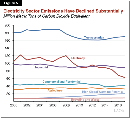
Electricity emissions reduced by 39 MMT (38 percent) from 2009 to 2017. During this same period, there was a net increase of more than 5 MMT from other sources of emissions.
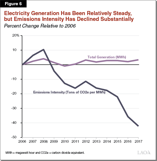
Overall Generation Relatively Steady, but GHG Intensity Has Declined Substantially. Total emissions from electricity depend on two basic factors: (1) total amount of electricity generated (megawatt hours, for example) and (2) the emission intensity (tons of CO2e per megawatt hour). As shown in Figure 6, total electricity generation has been relatively steady over the last decade, but emission intensity has declined by about 40 percent. Thus, it is a change in the mix of generation resources used to supply electricity that has been the primary driver of absolute emission reductions.
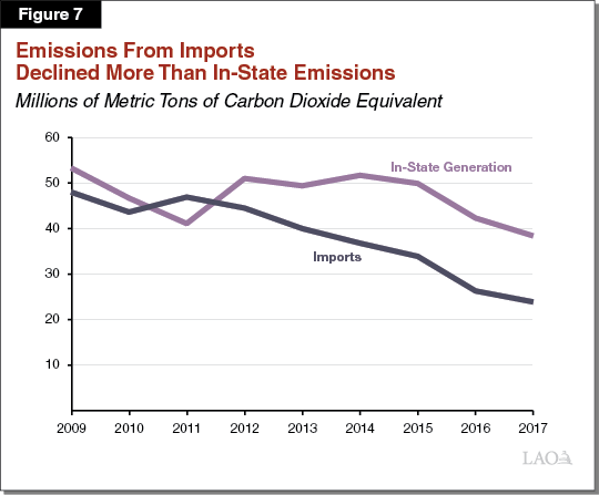
Most Declines Have Come From Imported Electricity. As shown in Figure 7, emissions from both in‑state generation and imports have declined since 2009, but imports have been the largest contributor to emission reductions. Overall generation from both in‑state generation and imports has been relatively steady. Most of the changes have been due to a reduction in emission intensity from imports, which has decreased by half since 2009.
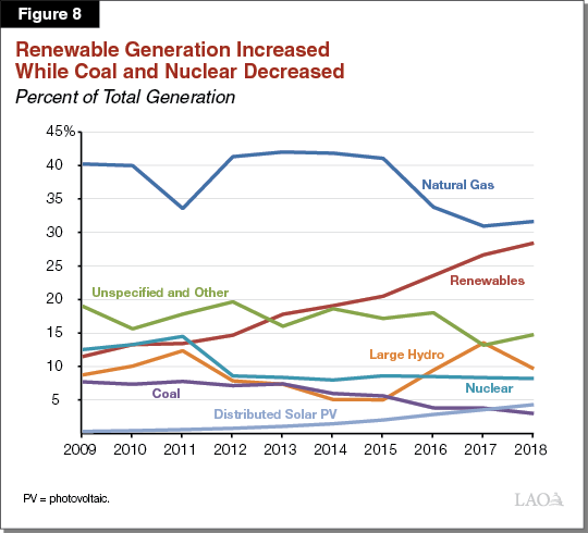
Renewables Increasing, While Coal and Nuclear Decreasing. Figure 8, illustrates changes in the total mix of generation sources since 2009 based on data from the CEC. The substantial increase in utility‑scale renewables is the most notable change over this period—the large majority of which was solar PV and wind. Distributed solar also increased substantially, even though the overall amount of generation is still relatively small. Generation from nuclear—a non‑GHG emitting source—and coal—a high source of emissions—have decreased in the last several years. Generation from natural gas, large hydroelectric, and unspecified sources have all varied over this time period. In the following section, we discuss the extent to which state policies have contributed to these changes.
LAO Assessment of Policies
As discussed in our 2018 report, Assessing California’s Climate Policies—An Overview, state policies have a wide variety of potential effects. These include:
- Benefits. Includes GHG reductions, reductions in criteria and toxic air pollutants, and promotion of activities—such as research and development—that create knowledge “spillovers” that have social benefits.
- Costs. Includes changes that increase the net cost of delivering electricity, including generation, transmission, and/or distribution. The increase in costs could also discourage businesses and households from undertaking valuable economic activities.
- Distributional effects. Includes instances when revenues or costs are shifted from certain households or businesses to others, without any net changes in economic costs or benefits.
In this section, we summarize our understanding of the major effects of California’s policies to reduce electricity emissions. Our assessment is based on a review of academic studies and various reports; our own analysis of data from government agencies and researchers; and conversations with various stakeholders, agencies, and researchers. The primary focus of our assessment is on the past effects of major policies, rather than projecting future effects of policies. In the following section, we identify and discuss key issues for future legislative consideration.
Policies Likely Substantial Drivers of Emission Reductions, but Actual Magnitude Unclear
Mix of Resources Used to Generate Electricity Has Lower Emissions. The changing generation mix described above has lowered emissions. For example, our simple “back‑of‑the‑envelope” estimate reveals that from 2009 to 2018, the increase in renewable generation reduced annual emissions by about 30 MMT of carbon dioxide—about 6 MMT from the increase in rooftop solar and 24 MMT from the increase in utility‑scale renewables. In addition, the decline in coal generation reduced annual emissions by about 8 MMT. These estimates are a rough proxy that do not take into account a wide variety of complicating factors, such as how a large addition of renewable generation capacity might affect the mix of other generation that was built and used. However, they provide a rough sense of the amount of GHG reductions associated with changes in the generation mix over the last few years.
State Policies Likely a Substantial Driver of Reductions . . . In total, state policies were likely substantial drivers of changes to the generation mix that lowered emissions. RPS and rooftop solar policies were almost certainly major factors in the significant expansion in renewable generation, particularly in early years when prices for this generation were much higher. (We discuss the price declines in more detail below.) In addition, SB 1368 was likely one factor that contributed to utilities divesting from coal power plants. Finally, by making high‑carbon electricity more expensive relative to low‑carbon electricity, cap‑and‑trade likely reduced the GHG intensity of electricity purchased by California LSEs.
. . . But a Wide Variety of Other Factors Also Likely Influencing Emissions. Although state policies were likely significant drivers of changes in electricity sector emissions, a wide variety of other factors may have also increased or decreased electricity emissions over the last several years. These include:
- Decline in Natural Gas Prices. Natural gas fuel prices decreased significantly over the last decade. Notably, prices declined by more than 50 percent between 2008 and 2009. As a result, natural gas generation might have replaced at least some of the coal generation even without state policy.
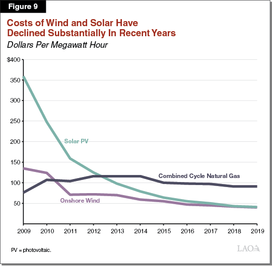
- Decline in Prices for Renewable Generation. As shown in Figure 9, the costs of unsubsidized renewable generation—particularly wind and solar—have declined substantially over the last decade. For example, global costs for utility‑scale solar PV declined by nearly 90 percent from 2009 to 2019. In recent years, LSEs likely would have purchased some renewable generation because it is less costly than other sources of generation, even if the state did not have an RPS policy. (As we discuss below, a small portion of the price decline might be driven by California policies, but much of the cost declines are likely driven by other global factors.)
- Federal Policies. The federal government offers tax credits for wind and solar that likely were factors contributing to the increase in renewables. For example, in 2006, the federal government implemented a solar investment tax credit offering a tax deduction of up to 30 percent of the cost of the solar system. The tax credit has been modified and extended a couple of times. Notably, there was originally a $2,000 cap on residential deductions that was eliminated in 2008. Certain federal environmental regulations that limit pollution from coal plants could also be factors affecting decisions to retire coal plants.
- San Onofre Nuclear Plant Stopped Operating. In 2012, one of the state’s two nuclear power plants stopped generating electricity due to safety concerns. This increased overall emissions since much of the zero‑carbon electricity had to be replaced by other sources of generation, including imports and natural gas generation. Based on other research that has been done and our own estimates, the closure increased annual emissions by about 7 MMT to 8 MMT annually.
- Annual Changes in Hydroelectric Generation. Hydroelectric generation is not likely a factor contributing to the long‑term trend in declining emissions because total hydroelectric capacity has not changed much over this period. However, hydroelectric generation varies from year to year based largely on the amount of rainfall in preceding years and, therefore, can be a significant factor affecting short‑term differences in emissions. For example, assuming natural gas as default, differences in hydroelectric generation over the last several years have changed annual emissions by about 10 MMT. One working paper estimates that the drought several years ago increased emissions by about 8 MMT annually.
- Voluntary Purchases of “Green” Electricity. Some households and businesses voluntarily choose to purchase low‑ or zero‑carbon electricity even if it is more expensive than alternatives. This can be done through Green Tariff programs offered through utilities, as well as by businesses that sign direct contracts with renewable electricity providers. This has likely driven some of the increase in renewable generation.
- Economic Recession. In 2008, California and the rest of the world suffered its worst economic recession in several decades. A reduction in economic activity tends to reduce emissions. In the electricity sector, we would expect a recession to largely affect overall electricity generation, rather than the mix of resources used to generate electricity. This is because electricity consumption (and generation) is likely more closely tied to changes in economic activity. Although the recession likely had an effect on emissions by reducing overall generation below what it would have otherwise been, it likely is not a significant driver of the decreases in electricity emission intensity. The economic growth over the last several years may have contributed to some growth in generation. However, similarly, it likely did not have much effect on the change in emission intensity.
- Resource Shuffling. Emissions leakage is when emission reductions that occur in California are offset by an increase in emissions in other states and countries. Resource shuffling is a specific type of leakage that occurs when—in response to state policies—more electricity generated from low‑carbon sources is sent to California, but more high‑carbon electricity is sent to other states. As a result, on paper, the electricity being used in California has lower emissions. However, the overall generation mix and total emissions throughout the western United States does not change. We discuss the potential for resource shuffling in more detail below.
No Rigorous Analysis of Overall Effects of State Policies. To our knowledge, there are no studies that have comprehensively evaluated the overall benefits, costs, and distributional effects attributable to state climate change policies in the electricity sector. Given the many different factors that affect California’s electricity emissions, it is difficult to attribute changes in emissions to any particular set of state policies. Such an analysis would likely require complex statistical modeling to estimate the effect of state policies. Furthermore, as we discussed in previous reports, there are significant interactions between state policies. For example, state policies that reduce emissions from sources that are covered by the cap‑and‑trade program—such as electricity sector policies that reduce emissions from in‑state generators and importers—might simply free up allowances for other sources to emit more. The net effect would be to simply change the source of emissions but not reduce the overall amount that would have been reduced if only cap‑and‑trade were in place. Even with the most sophisticated modeling tools available, it is unclear whether it would be possible to precisely estimate the total effect of California policies.
While there are significant challenges associated with evaluating the overall effects of state policies in the electricity sector, there is some information available about the effects of specific policies. Some policies have been evaluated by researchers using complex statistical techniques, while others have had almost no retrospective evaluation. Although there is not complete information on all the relevant effects of any particular policy, in some cases, the available data and research can provide valuable information about some of the major effects. In the next sections, we review the effects of the RPS, rooftop solar policies, SB 1368, and cap‑and‑trade.
RPS Likely a Significant Driver of Reductions At Moderate Costs Per Ton
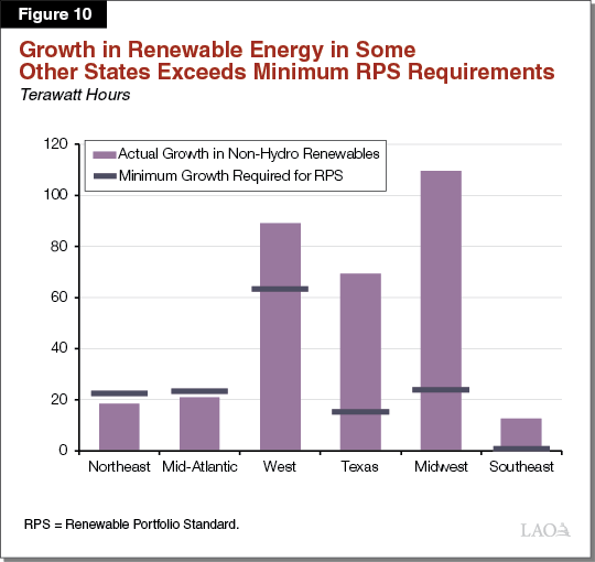
RPS Reducing State Emissions by Up to the Low Tens of Millions of Tons Annually. In general, LSEs have met or exceeded RPS requirements so far. According to CEC estimates, 34 percent of statewide retail sales in 2018 were met by RPS eligible resources. However, to our knowledge, there is no analysis of California GHG emission reductions directly attributable to RPS. As discussed above, our back‑of‑the‑envelope calculations suggest large‑scale renewables reduced emissions by roughly 24 MMT annually between 2009 and 2018. Many of these reductions are likely attributable to the RPS. However, for many of the reasons discussed above, it is difficult to isolate the effect of the RPS on the generation mix and emissions. Notably, some renewable generation would have been implemented even without the RPS as we have seen in other areas of the country. Figure 10 compares the growth in non‑hydroelectric renewable generation in different regions of the United States to the minimum growth required by state RPS policies in each region. In some regions—such as the Northeast and Mid‑Atlantic—growth in renewable generation is largely consistent with minimum RPS requirements in those states. On the other hand, growth in renewable generation for other regions—such as Texas, the Midwest—far exceeds RPS requirements. The renewable generation in these states has been driven by such things as lower unsubsidized costs for renewable generation (especially wind) and federal tax credits.
Properly accounting for these other factors would likely reduce the estimated emission reductions that are attributable to the RPS program. As a result, in our view, the estimate of 24 MMT of annual reductions is likely toward the high end of the range of likely emission reductions attributable to the RPS. It is also worth noting that we relied on total system generation data from the CEC to estimate renewable generation. However, there are key differences in accounting for renewable generation and GHGs between CARB, CEC, and CPUC. These add to the uncertainty of the estimate. We do not think these accounting differences would dramatically affect the magnitude of the estimates, but differences in accounting could change the estimates by several million tons annually.
Direct IOU Compliance Costs Likely Over $1 Billion Annually—Roughly 5 Percent of Total Costs. State law requires CPUC to report annually on IOU RPS procurement and generation costs, increases in total utility costs from meeting RPS requirements, and avoided costs as a result of meeting RPS. In total, CPUC estimates 2018 RPS procurement expenditures for the three large IOUs were $1.1 billion higher than alternative sources of electricity generation (the cost of a combined cycle natural gas power plant). Although this estimate is imperfect, it provides a rough sense of the RPS’s higher generation costs. For context, the large IOUs collect about $24 billion in annual revenue from “bundled” customers—or customers for whom the IOU procures the energy, as well as the distribution and transmission. The $1.1 billion in costs reflects an almost 5 percent increase in overall retail rates for bundled IOU customers. This increase is generally consistent with national studies that have found increased rates from RPS of about 3 percent to 8 percent.
As we discuss below, current RPS costs largely reflect long‑term renewable contracts that were signed several years ago when renewable prices—particularly for solar and wind—were much higher than they are today. These costs do not necessarily reflect future programmatic costs.
Back‑of‑the‑Envelope Calculations Suggest Moderate Direct RPS Costs Per Ton of Reductions. We are not aware of any retrospective evaluations of the cost per ton of reducing GHGs through the RPS. There are many challenges associated with making such an estimate. However, below we provide a back‑of‑the‑envelope calculation to provide a rough sense of the costs per ton—focusing on only the estimated differences in procurement costs.
Assuming RPS implementation by the large IOUs is responsible for about 60 percent to 70 percent of the reductions from 2006 to 2018, then RPS emission reductions from IOUs are about 17 MMT to 18 MMT in 2018. If direct procurement costs are about $1.1 billion higher, then the program is reducing emissions at a cost of roughly $60 to $70 per ton. We note that this is a rough calculation that excludes many factors, such as transmission and integration costs. This estimate also attributes all of the increase in renewable generation to the RPS, rather than other factors. As a result, we think this estimate reflects the low end of the range of costs per ton. Actual costs related to the RPS could be tens of dollars higher per ton.
For context, cap‑and‑trade allowance prices are currently about $17 per ton. In theory, this suggests that this program is encouraging emissions reductions that cost up to $17 per ton. In contrast, as we found in our 2018 report, Assessing California’s Climate Policies—Transportation, estimated costs for some of the transportation programs are much higher—hundreds of dollars per ton or more.
RPS Has a Wide Variety of Other Costs and Benefits. The RPS likely has other effects—both positive and negative—that are not captured in the estimates described above, which only reflect energy procurement costs. These include:
- Additional Transmission Costs. Utility‑scale renewable generation often requires new or upgraded transmission lines. Some national research has found that building transmission to wind and solar accounts for about 3 percent to 30 percent of overall costs of a project. However, the degree to which policies have affected transmission costs in California is not clear.
- Integration Costs. Regulators and grid operators must ensure there are enough other resources available to supply energy (and other related grid services) when demand increases or the supply of intermittent renewables decreases. This could include payments to natural gas generators to make sure they are available in case they are needed to balance the grid and the costs of paying for electricity storage so it can be used during other times when the renewable sources are not producing as much energy. To our knowledge, there has been no complete retrospective evaluation of these integration costs in California. Some national research has estimated that integration costs are similar to transmission costs described above—about 3 percent to 30 percent of total project costs. These costs are likely lower in earlier years with low percentages of intermittent renewables, but can increase substantially as the percentage of renewables grows.
- Reduced Local Air Pollution. Replacing coal and natural gas generation with certain renewables—such as wind and solar—reduces other local air pollutants. (It is less clear how an increase in other renewables, such as biomass, affect total nitrogen oxide [NOx] emissions.) Using a back‑of‑the‑envelope calculation, we estimate the increase in wind and solar generation reduced about 8,000 tons of NOx and 1,000 tons of particulate matter (PM2.5) in 2018. For context, this is a relatively small reduction compared to total statewide annual emissions—less than 2 percent for NOx and less than 1 percent for PM2.5. Plus, some of these reductions come from generators in other states so do not affect air quality in California. It is also worth noting that some studies have found that the RPS benefits from local air pollution reductions meet or exceed the benefits of GHG reductions in other states. However, the largest local air pollution reductions occur in states that rely heavily on coal. The local air pollution benefits of an RPS are generally lower in California because the mix of existing generation that is being displaced (mostly natural gas) generates much less local air pollution.
- Contribution to Decline in Solar Prices. As discussed above, costs for renewables—and solar PV in particular—have declined substantially over the last decade. The decline in costs of installing solar PV largely have been driven by a decline in the costs for the solar panels (also known as modules). California policies likely partially contributed to the declining price of solar panels. For example, as a result of the additional production of solar panels driven by California policies, manufacturers could have learned how to produce the panels more efficiently—also known as “learning‑by‑doing” (LBD). Other firms might then learn these techniques for reducing production costs and, as a result, the market price for solar panels declines. However, it is important to note that solar panels are produced and sold in a global market and the degree to which California policies—relative to other global factors—affected those prices is unclear. Given the scale and timing of some of California’s activities relative to those that occurred in other jurisdictions—such as Germany, China, and Japan—California policies are likely a relatively minor driver of these reductions. For example, solar PV capacity in California is only a few percent of global PV capacity. That said, even a small contribution to the substantial decline in prices could have significant global benefits.
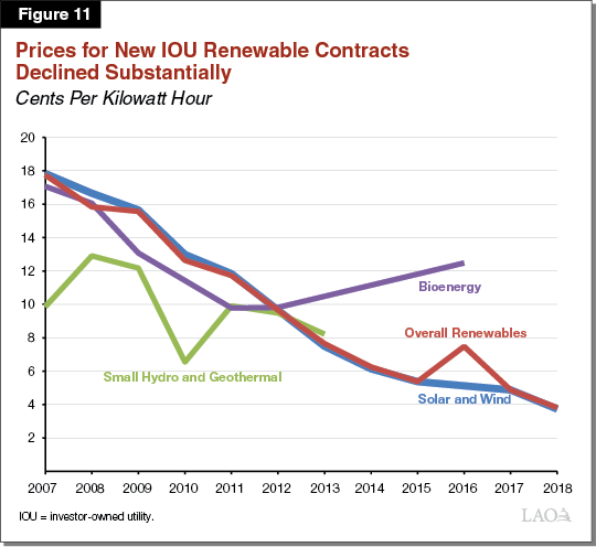
Future Program Costs Could Be Much Different Than Past Costs. As discussed above, global costs to install renewable energy have decreased substantially in recent years. Figure 11 shows how prices for new IOU RPS contracts—particularly wind and solar—have declined over time. The costs for certain types of renewable energy—particularly solar PV—under these more recent contracts will be lower than they have been in the past. Since 2007, the only increase in overall renewable contract prices was in 2016 which was primarily due to an increase in contracts for biomass electricity (one type of bioenergy) in response to a legislative mandate to procure a certain amount of biomass capacity. These contracts were more expensive than recent wind and solar contracts.
While procurement costs for renewables is likely to decline, as the percentage of intermittent renewables used for generation grows, integration costs are likely to increase. The net effect of these changes depends on the future trends in renewable costs and the costs of different strategies to manage intermittency (storage costs, for example).
Rooftop Solar Policies Generally More Costly
The state has implemented several different policies aimed at increasing adoption of distributed solar—primarily rooftop PV—as a way to reduce GHGs. In this section, we focus on two key policies that have been used to increase adoption—the CSI and NEM—as well as some of the effects of rooftop solar more generally. Relative to the other climate policies that we reviewed in this report and in previous reports, there has been a significant amount of retrospective evaluation of the effects of some of the state’s rooftop solar policies. In particular, there is a robust literature on the effects of the CSI. We summarize the key findings about CSI and NEM below.
CSI Increased Adoption of Rooftop Solar, but Significant Portion of Rebates Went to “Free‑Riders.” As discussed earlier, total distributed solar PV generation reduced annual emissions by up to 6 MMT in 2018. Academic studies consistently find that the CSI rebates offered for solar installations were mostly or fully passed through to consumers in the form of lower prices for the solar installations, rather than increasing profit for businesses selling the units. Furthermore, studies consistently find that the CSI increased rooftop solar adoption relative to a scenario where no CSI rebates were offered.
However, these studies also found that a large portion—sometimes 50 percent or more—of the households that installed solar would have purchased rooftop solar without the CSI rebate. Such consumers are sometimes known as free‑riders. This finding is consistent with research related to other programs that offer rebates for new technologies—such as hybrid electric vehicles—that finds a high proportion of rebates go to free‑riders.
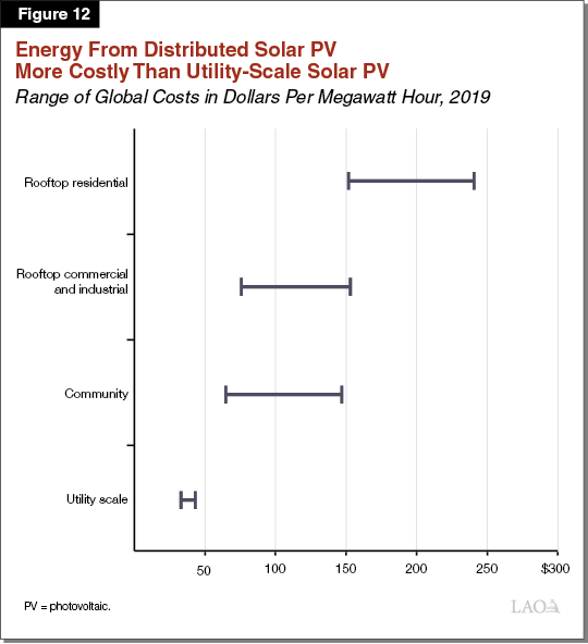
Rooftop Solar Much More Costly Than Utility‑Scale Solar. There has been a significant decline in the cost of installing distributed solar PV. However, as shown in Figure 12, recent estimates of the costs of generating electricity from different solar PV sources shows that distributed solar PV is much more expensive than utility‑scale solar PV. For example, rooftop residential solar PV is about five times more costly than utility‑scale solar PV. Commercial and industrial rooftop solar is about two to three times more expensive than utility scale. Although these are global cost estimates that are subject to a wide variety of limitations and uncertainties, they suggest that there is a large difference in the costs of installing and generating energy from distributed solar compared to utility‑scale renewables. The difference in cost could be due to a variety of factors, including higher installation costs per unit for rooftop solar due to economies of scale and greater ability to install utility‑scale solar in locations that have the most sunlight to maximize generation.
CSI Costs Likely Significantly Higher Than RPS. In addition to the differences in costs described above, a few studies estimated the costs of CSI specifically. For example, two studies found that the CSI rebates reduced GHG emissions at a program cost of about $150 to $200 per ton. These estimates are higher than the $60 to $70 per ton estimates for RPS described above. It is worth noting that—similar to the RPS—these estimates generally do not include any program benefits or costs related to knowledge spillovers, improvements in local air pollution, or other effects on the grid.
Overall Effects of NEM Less Clear but Results in Substantial Cost Shift to Nonsolar Customers. To our knowledge, there have been no retrospective evaluations of the overall GHG reductions and/or economic costs from NEM. However, one aspect of the NEM program that has been evaluated is the degree to which the program shifts costs from solar customers to nonsolar customers. The key mechanism by which NEM provides financial incentives for customers to install distributed generation is through shifting fixed costs from solar customers to nonsolar customers. This occurs because—for each unit of rooftop solar generation—solar customers no longer pay the retail rate for utility‑generated electricity that includes fixed costs for the transmission and distribution systems. When solar customers no longer pay for these fixed costs, these costs are generally built into the electricity rates paid for by other (nonsolar) customers. It is important to note that changing who pays for fixed costs that have already been incurred is not considered a net economic cost, but can have significant distributional implications.
One rough estimate by an economist at the University of California found that the additional costs borne by nonsolar customers is about $65 per customer annually. Another evaluation found that the benefit to the solar customer of the cost shift was about $1,200 annually for two of the largest IOUs in 2016. This study also found that the total amount of the cost shift for each utility was a few hundred million dollars annually. This amount grows over time as the amount of rooftop solar grows and if utilities incur additional costs for distribution and transmission. Importantly, CPUC recently modified NEM and required that new NEM customers enroll in TOU pricing. This change—at the time it was adopted in late 2016 and early 2017—was expected to reduce a solar owners’ overall financial benefit of generation during “off‑peak” hours—such as hours in the middle of the afternoon when rooftop solar generation is relatively high but retail prices are lower under TOU rates. However, this is partially offset by an increase in the benefit during some of the peak hours—such as in the late afternoon—when solar PV is still generating and TOU rates are higher. On net, these changes are likely to reduce the overall financial benefit to customers from NEM. These changes also reduce the amount of the cost‑shift to nonsolar customers.
Recent Study Finds Small LBD Benefits. One common rationale for California’s rooftop solar policies—including CSI and NEM—is LBD, whereby the cost of a technology declines with more cumulative experience with the technology. If there are learning spillovers—where, for example, one firm learns how to install solar more efficiently but other firms also learn from that experience—then there could be an economic rationale for government policies that encourage greater deployment of new technologies. (This is similar to the justification for governments funding research and development to create knowledge that is publicly available.) Most of the potential LBD benefits for rooftop solar programs are likely to occur for what are known as balance of system (BOS) costs—or costs related to the installation of the solar panels, rather than the costs of the equipment. At least a few different studies have estimated the degree to which CSI has led to learning‑by‑doing for solar BOS costs—one as the program was beginning and two after the program was implemented.
- 2008 Prospective Study Found That Primary Benefit From CSI Was LBD . . . One 2008 study found that LBD benefits were roughly ten times greater than the direct environmental benefits associated with the CSI. The study found that, without LBD benefits, environmental benefits did not justify CSI subsidies. However, assuming a certain level of LBD benefits, the level of CSI rebates were close to optimal.
- . . . But Retrospective Studies Find Small LBD Effects. More recent research has found very weak evidence of LBD benefits from 2002 to 2012, and the magnitude of effect was relatively small. During the study period, BOS costs declined by less than $1 per watt ($3 per watt to a little more than $2 per watt). Over a similar time period, hardware costs declined from over $7 per watt to less than $3.5 per watt. Only 15 percent ($0.12) of the decline in BOS costs were found to be attributable to LBD. Further, there was evidence of only very small learning spillovers, at least in the short run. Another study found that LBD contributed to a 5 percent decrease in solar prices, which is a clear benefit but relatively small compared to the 33 percent decrease in solar prices over the entire period of the study.
Little Evidence of a Substantial Reduction in Distribution Costs, Except in Certain Locations. Some stakeholders argue that rooftop solar reduces a utility’s costs associated with building out its distribution network. In theory, this could occur because it reduces the demand on the system during peak hours of electricity demand, thereby reducing or delaying the need for the utility to add potentially expensive distribution capacity. Other potential benefits include potentially reducing the amount of “line‑loss,” or the electricity lost as it travels through the grid system, because the electricity does not have to travel as far. However, an increase in rooftop solar also has the potential to add distribution costs. This could occur because adding distributed solar sometimes can require modifications to the existing distribution network to accommodate the new generation sources being connected to the grid. In total, therefore, the overall magnitude—and even the direction—of the effect of adding distributed solar on distribution costs is not obvious.
The research on the effects of distributed solar on distribution costs is somewhat limited but shows mixed results. One study found that the net costs depend on various factors including how much other local distributed solar PV exists, as well as certain other characteristics of the distribution grid at the specific location. The same study found that there was very little benefit associated with reducing “congestion” on most distribution circuits, but there was substantial value on 1 percent of circuits. The value is especially significant in areas where circuits are very close to needing a capacity upgrade. Another working paper (which focused only on the costs to modify the existing network but not potential avoided or delayed costs) found that (1) the vast majority of a 100 percent increase in average residential distribution network prices between 2003 and 2017 can be explained by the increase in distributed solar generation and (2) larger amounts of rooftop solar that is more concentrated geographically predict higher distribution network costs.
Rooftop Solar Has Other Advantages Over Utility‑Scale, but Magnitude of Benefits Unclear. There are some other areas where rooftop solar has clear advantages over utility‑scale solar. For example, one common rationale for encouraging rooftop solar is because it has fewer land use impacts than utility‑scale solar installations that require acres of land, which sometimes require the conversion of natural and working lands. We did not identify any research that quantified the magnitude of this potential benefit, but it could be significant. Another potentially substantial benefit is that distributed solar could provide enhanced electric reliability during electric power shutoffs that are being implemented to reduce the risk of wildfires, particularly when distributed solar is accompanied by battery storage. While it is clear such advantages might exist, the magnitude of these benefits—and the degree to which state policies might be needed to help promote these actions—are unclear.
Little Known About Effects of SB 1368 and Cap‑and‑Trade
No Empirical Research on the Effects of SB 1368. Since 2009, coal generation for California has declined by over 60 percent and now makes up only 3 percent of the state’s electricity supply mix. We did not identify any retrospective empirical research that identified the degree to which SB 1368 contributed to this decline. Based on conversations with various stakeholders, it is likely that the policy was a significant factor contributing to the decline in coal generation. However, other factors—such as declines in natural gas prices and cap‑and‑trade—were also likely important.
Level of Cap‑and‑Trade Costs More Clear Than Level of Emission Reductions. Allowance prices are an indicator of the marginal costs for emission reductions encouraged by the cap‑and‑trade program. Since the cap‑and‑trade program began in 2013, electricity generators and importers have had to pay a carbon price of roughly $10 to $17 per ton. In theory, if lower‑carbon electricity can be provided for a net difference in costs of less than $17 per ton, then the lower‑carbon electricity will be generated in or sent to California.
The emission reductions associated with the program are more difficult to estimate. Carbon prices have been incorporated into wholesale electricity market bids, which at times has likely resulted in lower carbon mixes of electricity supply being purchased in the market than would otherwise have been the case. It is also possible that expectations about future carbon prices have affected LSE long‑term procurement decisions. However, to our knowledge, there has not been any empirical research estimating these effects. Based on conversations with stakeholders and researchers, the effect on electricity sector emissions is generally thought to have been relatively modest compared to other policies, such as RPS. As emissions targets become more ambitious in future years, cap‑and‑trade could result in significantly higher costs and emissions reductions associated with electricity generation.
Allocating Free Allowances to IOUs Under Cap‑and‑Trade Has Benefited Ratepayers. As discussed in our 2018 report Assessing California’s Climate Policies—An Overview, some of the most visible effects of the cap‑and‑trade program are not net economic costs, but what are known in economic terms as transfers. For example, the cost of purchasing allowances—also known as compliance costs—is generally not considered a net economic cost. Instead, the purchase of allowances results in a transfer of money from the entity who ultimately bears the cost of purchasing the allowances to those who get the revenue from selling the allowances. In the electricity sector, electricity generators and importers are directly responsible for purchasing allowances, and those costs are generally passed on to utility consumers in the form of higher electricity rates.
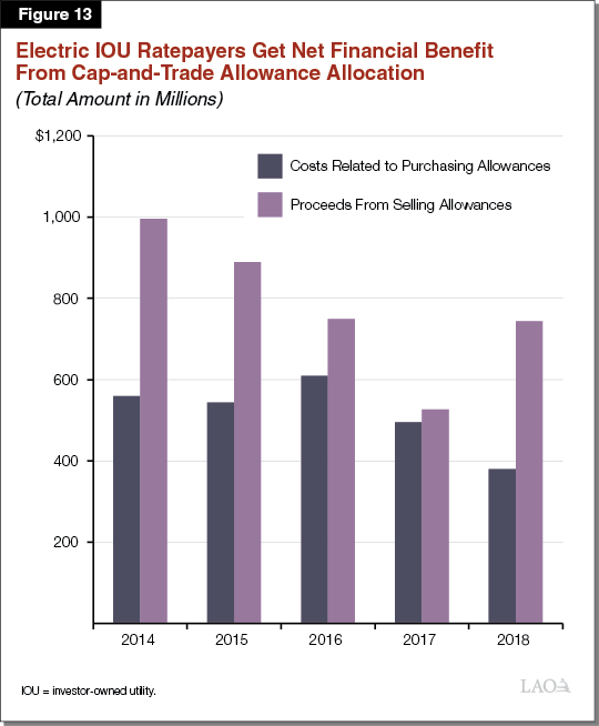
While ratepayers bear costs associated with cap‑and‑trade for the electricity they use, the state provides free allowances to IOUs that they sell and use the revenue to benefit ratepayers. The large majority of this revenue is used to provide a semiannual bill credit to residential customers. As shown in Figure 13, compliance costs for IOU ratepayers are far less than the amount of IOU proceeds from the sale of allowances going to IOU ratepayers. It is important to note that the amount of allowance revenue that goes to benefit ratepayers is also used to provide bill credits for CCA and ESP customers, but the compliance costs do not include costs for CCA and ESP customers. However, even after adjusting for this difference, this data suggests that electric ratepayers have, on average, benefited financially from the economic transfers that occur under the program. It is also important to note that the effect of cap‑and‑trade on consumers of other fuels—such as transportation fuels—is likely much different because businesses and consumers in those sectors do not receive as many free allowances.
Resource Shuffling Potentially Offsets Some of the Emissions Reductions
Resource shuffling occurs when, in response to California climate policies, the mix of existing electricity supplies changes so that more low‑carbon electricity is sent to California while more high‑carbon electricity is sent to other states. To the degree this occurs, the reduction in the carbon intensity of California’s electricity supply would not actually reflect a net reduction in low‑carbon generation. Understanding the degree to which resource shuffling has occurred is an important factor in identifying the net effect California policies have had on overall GHG emissions. Resource shuffling could be driven by a wide variety of policies in the electricity sector, but it is especially relevant for SB 1368 and cap‑and‑trade.
Different Potential Mechanisms for Resource Shuffling or Leakage. As outlined in a 2018 report from the state’s Independent Emissions Market Advisory Committee (IEMAC), there are several different mechanisms through which state policies could contribute to leakage or resource shuffling in the electricity sector. These include:
- Bilateral Contract Shuffling. California entities will no longer enter into bilateral long‑term contracts with coal power plants, but these coal plants might continue to operate and sell to entities in other states instead, thereby not resulting in a decrease in total electricity generation from coal.
- Regional Electricity Markets. In short‑term wholesale markets where electricity is dispatched based on lowest cost, low‑carbon energy is delivered to California to avoid the state’s carbon price while high‑carbon energy is sent to other states.
Research Shows Potential for Significant Resource Shuffling, but Not Much Retrospective Evaluation. As discussed above, many of the emission reductions in the electricity sector have come through reduced emissions intensity of imports. Several different prospective analyses showed that there was potential for significant resource shuffling. For example, as a result of SB 1368 and/or cap‑and‑trade, coal power plants that no longer send electricity to California could provide electricity to other states, while lower‑carbon sources of electricity (such as hydroelectric) would be sent to California. Some of these studies estimated the magnitude of resource shuffling could be at least several million tons annually.
To our knowledge, however, there has been very little retrospective empirical research estimating resource shuffling. As a result, the degree to which resource shuffling has actually occurred is highly uncertain. The only empirical research we are aware of is a working paper that found emissions decreased by 12 million tons annually in California and increased by about 8.5 million tons in other parts of the western United States after cap‑and‑trade was implemented. This suggests about 70 percent of emission reductions leaked out of state.
Summary of Findings
Figure 14 summarizes the key findings from our review of the effects of the state’s major climate policies affecting the mix of electricity generation.
Figure 14
Summary of Findings
|
Policies likely substantial driver of emission reductions, but actual magnitude is unclear.
|
|
Renewable Portfolio Standard (RPS) likely a significant driver of emission reductions at relatively moderate costs per ton.
|
|
Rooftop solar policies generally more costly emission reduction strategy.
|
|
Little known about overall effects of SB 1368 and Cap‑and‑Trade.
|
|
Resource shuffling potentially offsets some of the observed emission reductions.
|
Key Issues for Legislative Consideration
The prior section summarizes key findings from our review of the effects of policies that have been implemented so far. In this section, we discuss some of the key issues for the Legislature to consider going forward as the state modifies and adopts policies to achieve its GHG goals. Specifically, we identify considerations related to facilitating future policy evaluations, promoting cost‑effectiveness, and reducing barriers to long‑term electrification.
Comprehensive Policy Evaluations Lacking
As described above—and similar to findings in our 2018 report on transportation policies—we found a lack of rigorous retrospective evaluations of the major effects of some of the state’s climate policies related to electricity generation. Below, we provide options that the Legislature might want to consider to help ensure more robust evaluation of state climate policies in the future. Findings from these evaluations could help inform the Legislature’s future policy and budget decisions, as well as provide valuable information for other jurisdictions considering adopting similar policies intended to reduce GHG emissions.
Consider Directing Agencies to Identify Opportunities to Facilitate Retrospective Evaluation. Agencies can help facilitate retrospective evaluation by ensuring data are available to researchers and, potentially, designing programs in ways that allow for more robust evaluations. The CSI is an example of a program that had both of these features and, as a result, there is a significant amount of information about the program’s effects. First, the program collected—and made publicly available—a lot of data about the amount of solar generation that was installed under the program. Second, some specific features of the program were structured in a way that facilitated more robust evaluation. For example, rebates varied across time and location depending on the amount of solar that had already been installed in a utility’s service territory. This variation allowed researchers to utilize research methods that could better identify which solar installations were attributable to the CSI versus other factors.
Similar to our comments in previous reports, the Legislature might want to consider directing agencies to identify opportunities to help facilitate better retrospective evaluation before programs are adopted or modified. This planning process could include requiring implementing agencies to develop a research plan for the program that would identify, for example, what data would be collected and how the program could be designed to help facilitate retrospective evaluation. The Legislature also might want to consider directing state agencies to consult with academic researchers during this process.
RPS Reports Might Be Guide for Other Climate Programs With Potential for Some Improvements. Much of the information on the effects of the RPS was based on multiple reports that were required from CPUC on an annual basis. One of these reports focuses on progress in complying with the RPS requirements. Another focuses on the costs associated with RPS procurement. These reports provide helpful information on the past and current effects of the program. Most notably, the cost report includes an estimate of what energy expenditures would have been without the RPS. Although imperfect, the estimate provides helpful information on the costs associated with the program compared to a scenario where the RPS did not exist. We are not aware of similar state reporting requirements for many of the other major climate policies (including some of the state’s major transportation policies, which we discussed in our report last year). The Legislature might want to consider whether similar requirements could be implemented for other climate programs.
Although CPUC’s RPS reports provide valuable information, there might be opportunities to improve them. For example, there are additional RPS costs—including transmission costs and integration costs—that are not included in the report. The Legislature might want to require more reporting on RPS related to these costs. Although more difficult to estimate, these costs—particularly the integration costs—could be a substantial part of the overall costs of implementing RPS in future years. Additional information on these costs could help inform future legislative decisions about potential changes to the program. In addition, the current RPS reporting requirements do not require CPUC to estimate the GHG emission reductions associated with the program. The Legislature might want to require CPUC to report on the estimated GHG benefits of the program since emission reductions is the primary goal of the program.
Other Future Reporting and Research Priorities. Some of the key areas where the Legislature might want to consider additional reporting requirements and/or funding for research efforts include:
- Resource Shuffling. Evaluation of resource shuffling is particularly important since many of the emission reductions have come from imports, and there is a body of research that suggests resource shuffling could be a significant factor. The degree to which it has occurred is still unclear though. The 2018 Annual Report of the IEMAC noted some key challenges associated with accurately estimating resource shuffling, and it provided recommendations intended to improve monitoring and mitigation. These included such things as better harmonization of data between CARB, CEC, and CPUC. The Legislature might want to consider requiring some of those changes in order to facilitate greater evaluation.
- Effect of Distributed Solar on Distribution Costs. As discussed earlier, rooftop solar can have costs and benefits related to the distribution grid. Some of these effects have been studied, but additional evaluation of these effects could be particularly valuable to inform future decisions related to distributed solar. For example, to our knowledge, very little is known about the degree to which—or where—distributed solar has reduced costs by delaying the need to make distribution infrastructure upgrades. The Legislature might want to consider directing CPUC to evaluate these effects in more detail.
Mix of Policies Likely Not Most Cost‑Effective Way to Reduce GHGs
As the state’s GHG goals become more stringent, the overall costs to reduce emissions is likely to grow. The higher costs are likely driven by (1) greater annual emission reductions needed to meet the target are higher because the reduction targets are more aggressive and (2) the cost per ton of reducing emissions increases as the low‑cost emission reduction actions—or the “low hanging fruit”—have already been taken. As a result, cost‑effectiveness becomes increasingly important.
Based on our review of the available information, there has been substantial differences in the costs of reducing emissions between cap‑and‑trade (marginal cost that are currently less than $20 per ton), RPS (average costs of about $60 to $70 per ton or more), and distributed solar policies (average costs of roughly $150 to $200 per ton). In the future, the Legislature might want to consider relying more heavily on the most cost‑effective programs, such as cap‑and‑trade.
There might be instances where there is a strong rationale for supporting policies that are not the most cost‑effective in the short term, but that provide other important benefits. For example, some policies, such as those that promote innovation or LBD by supporting new technologies, might have significant long‑run benefits by creating knowledge spillovers. Some targeted state policies focused on the development of technologies that could help achieve those goals might be warranted. The focus of such efforts could include (1) technologies that are in earlier stages of development but that might end up being valuable to help meet long‑term GHG goals, (2) technologies where increase in deployment is more likely to result in LBD spillovers, and (3) technologies that are more likely to be adopted in other jurisdictions. Another example, is policies that result in significant reductions in local air pollutants. In some cases, the Legislature might want to consider adopting policies that are a somewhat more costly way to reduce GHGs if those policies result in substantially greater reductions in local air pollution. Ultimately, the Legislature will have to balance the higher costs against some of these other benefits, which can be difficult to quantify in some cases.
High Electricity Prices Could Be Barrier to Future Emission Reductions
As the state’s GHG targets become more ambitious and new technologies are deployed more widely, it will become increasingly important for the state to consider relationships across different sectors. In other words, consider how policies in one sector—such as electricity—affect emissions in other sectors—such as transportation fuels and fuels for home appliances. One important example of this relationship is how electricity rates affect incentives to electrify other parts of the economy. We discuss this issue in more detail below.
California Rates Are Significantly Higher Than Most Other States. Retail electricity rates in California are generally much higher than many other areas of the country. For example, the average rate in California in 2017 was about 16 cents per kwh, or about 50 percent higher than the national average of roughly 10 cents per kwh. Rates vary among LSEs. For example, rates for the three largest IOUs range from 16 cents to 24 cents per kwh.
Wide Variety of Factors Contributing to High Rates. Some of the factors that contribute to California’s comparatively high retail electricity prices include:
- How Fixed Costs Are Recovered. One key factor affecting electricity rates is how a utility collects revenue to cover fixed costs for transmission and distribution. Generally, California IOUs recover their fixed costs through volumetric rates, thereby increasing per kwh rates paid by customers. Utilities in other parts of the country often collect more of their fixed costs through monthly fixed charges.
- Declining Consumption. All three large IOUs have had declining retail electricity sales in recent years, at least partly driven by increases in distributed solar generation (which decreases the amount of electricity purchased from the utility) and improvements in energy efficiency. Since fixed costs are largely recovered in volumetric rates, then declining electricity consumption can increase electricity rates. With fewer retail sales, higher electricity rates are needed to raise the same amount of revenue to cover fixed costs.
- State Program Costs. A wide variety of state policies and programs also increase electricity rates for an average California customer. This includes policies discussed earlier in this report—such as RPS, cap‑and‑trade, and policies that promote distributed generation—as well as a wide variety of other policies to promote energy efficiency, fund electric vehicle infrastructure, and provide subsidized rates for low income customers.
High Retail Rates Could Make It More Difficult to Achieve Long‑Term GHG Goals. There is nothing inherently wrong with having rates that are higher than other states. For example, if the rates reflect the true social costs of providing an extra unit of electricity (including environmental damages), then the prices might be appropriate. However, based on findings from a recent working paper, electricity rates in California are more than twice as much as the marginal social costs of providing electricity in California, even after accounting for environmental damages.
Rates that are much higher than the social marginal costs have adverse economic effects because they discourage valuable economic activities that might have otherwise occurred. For example, high rates might make it more expensive for a business to produce valuable goods and services in California. Similarly, households might avoid electricity consumption that is valuable to them, such as setting the home thermostat at a more comfortable temperature.
Furthermore, high electricity rates could present a barrier to long‑term emission reductions. Although high electricity rates might encourage some emission reduction in the electricity sector through reduced consumption and greater efficiency, they serve as a barrier to GHG reductions in other sectors. For example, one strategy for substantially reducing statewide GHGs is electrification—or using low‑carbon electricity to power vehicles and provide heat in buildings. This includes using electric vehicles instead of gasoline‑powered cars. It could also include using electric appliances—such as electric heat pumps and water heaters—in place of appliances powered by natural gas. Decisions by households and businesses about whether or not to adopt these alternative technologies depend, in part, on electricity rates. Higher electricity rates could discourage some adoption of these lower‑carbon technologies. The relative weight given to energy efficiency compared to electrification of other sectors might depend, in part, on whether the Legislature’s primary focus is on incremental near‑ to medium‑term reductions, or whether the primary goal is long‑term decarbonization. Although energy efficiency can potentially help reduce emissions in the near‑ to medium‑term, the state cannot reach substantial economywide decarbonization with only energy efficiency. It must adopt other low‑ or zero‑carbon sources of energy for all sectors of the economy. Electrification of a substantial portion of other sectors, along with a decarbonized electricity grid, is one of the strategies most often discussed for achieving those types of substantial GHG reductions.
Consider Retail Rate Structures That More Closely Reflect Marginal Costs of Electricity. The Legislature might want to consider actions that encourage LSEs to adopt retail electricity rates that more closely reflect the marginal costs of providing the electricity. For example, the Legislature could direct CPUC to exclude at least some of the fixed costs and certain state policy costs from IOU volumetric electricity rates. From an economic perspective, this would improve efficiency by making rates more closely reflect the marginal social costs of providing the electricity. From a GHG perspective, the lower volumetric rates would reduce the incentive for energy conservation and energy efficiency, but would make it more financially attractive for households and businesses to purchase electric vehicles and appliances.
Reduced Revenue From Lower Rates Could Be Made Up in Other Ways. If at least some fixed grid costs or state policy costs are removed from electricity rates, the state would have to determine who pays for those costs and how. A couple of potential solutions are:
- Fixed Charges. The state could direct utilities to increase the use of fixed monthly charges for electricity customers to pay for fixed grid costs. One of the primary concerns with this approach is that it might shift a greater portion of the fixed costs to households that tend to consume less electricity, including low‑income households. One potential solution to this concern would be to assess lower fixed charges for low‑income customers.
- Other Funding Sources. The state could consider using other funding sources to pay for costs for certain programs that are aimed at achieving statewide policy goals, such as deployment of electric vehicle infrastructure. Since many of these programs are aimed at promoting statewide public policy goals, there is a rationale for using state budgetary resources to cover the costs, including the General Fund and Greenhouse Gas Reduction Fund (which gets funding from auctions of the state’s cap‑and‑trade allowances). The Legislature could also direct the utilities to use revenue from the sale of their cap‑and‑trade allowances to pay for some of these programs.
Each of these options involves its own set of implications and trade‑offs that would need to be carefully examined. For example, using other state funding sources would require a reduction in funding for other state programs and/or additional revenue collected from taxpayers. Each of these has trade‑offs that would need to be balanced against the potential ratepayer and emission reduction benefits related to lower electricity rates.
Conclusion
The state’s climate policies in the electricity sector are complex and have a wide range of effects—both positive and negative. Based on our review, some of our main findings include: (1) state policies are likely a substantial driver of emission reductions, but the overall magnitude of the effect is unclear; (2) the RPS program is likely a significant driver of emission reductions at relatively moderate costs per ton, (3) rooftop solar policies are generally a more costly emission reduction strategy, but could provide significant benefits in certain instances; (4) relatively little is known about the overall effects of SB 1368 and the benefits from cap‑and‑trade; and (5) resource shuffling could potentially offset some of the observed emission reductions. We also identify a variety of issues for the Legislature to consider going forward as the state modifies and adopts policies to achieve its GHG goals. These issues include program evaluation, cost‑effectiveness, and how high electricity rates could potentially serve as a barrier to long‑term GHG reductions.
Appendix
Selected References
Barbose, G (2019). “U.S. Renewable Portfolio Standards: 2019 Annual Status Update.” Lawrence Berkeley National Laboratory.
Bollinger, B. and K. Gillingham (2019). “Learning‑by‑Doing in Solar Photovoltaic Installations.” Working paper, April 3 version.
Borenstein, S., and J. Bushnell (2018). “Do Two Electricity Pricing Wrongs Make a Right? Cost Recovery, Externalities, and Efficiency.” Natural Bureau of Economic Research. Working Paper No. 24756.
Bushnell, J., Y. Chen, and M. Zaragoza‑Watkins. (2014). “Downstream regulation of CO2 emissions in California’s electricity sector.” Energy Policy 64: 313‑23.
California Public Utilities Commission (2019). “2019 Padilla Report: Costs and Savings for the RPS Program.”
California Energy Commission (2018). “Tracking Progress: Renewable Energy.” Updated December 2018.
Cohen, M.A., B.A. Kauzmann, and D.S. Callaway (2016). “Effects of distributed PV on California’s distribution system, part 2: Economic analysis.” Solar Energy 128: 139‑152.
Cullenward, D. (2014). “Leakage in California’s carbon market.” Electricity Journal 27(9): 36‑48.
Davis, L. “Why Am I Paying $65/year for Your Solar Panels?” Energy Institute Blog, UC Berkeley, March 26, 2018.
Gorman, W., A. Mills, and R. Wiser (2019). “Improving estimates of transmission capital costs for utility‑scale wind and solar projects to inform renewable energy policy.” Energy Policy. Pre‑print.
Hughes, J.E and M. Podolefsky. 2015. “Getting Green with Solar Subsidies: Evidence from the California Solar Initiative.” Journal of the Association of Environmental and Resource Economists. Volume 2, Number 2: 235‑275.
Independent Emissions Market Advisory Committee (2018). “2018 Annual Report of the Independent Emissions Market Advisory Committee.”
Lazard (2019). “Lazard’s Levelized Cost of Energy Analysis—Version 13.0.”
Lo Prete, C., A. Tyagi, and C. Hohl (2019). “California’s Cap‑and‑Trade Program and Emissions Leakage in the Electricity Sector: An Empirical Analysis.” Manuscript in preparation. July 3rd version.
Mastrandrea, M.D., M. Inman, and D. Cullenward (2019). “Assessing California’s progress toward its 2020 greenhouse gas emissions limit.” Pre‑print. https://doi.org/10.17605/OSF.IO/FE25W
Rogers E. and S. Sexton (2015). “Effectiveness of Capacity‑Dependent Rooftop Solar Subsidies: Lessons from California.” American Economic Association’s Annual Meeting: Allied Social Science Associations Program. Presentation on January 3rd.
Sergici, S., Y. Yang, M. Castaner and A. Faruqui (2019). “Quantifying net energy metering subsidies.” The Electricity Journal (32) 106632.
Van Bentham, A., K. Gillingham, and R. Sweeney (2008). “Learning‑by‑Doing and the Optimal Solar Policy in California.” The Energy Journal 29(3): 131‑151.
Wiser, R., G. Barbose, J. Heeter, T. Mai, L. Bird, M. Bolinger, A. Carpenter, G. Heath, D. Keyser, J. Macknick, A. Mills, and D. Millstein (2016). “A Retrospective Analysis of the Benefits and Impacts of U.S. Renewable Portfolio Standards.” Lawrence Berkeley National Laboratory and National Renewable Energy Laboratory. NREL/TP‑6A20‑65005.
Wolak, F. (2018). “The Evidence from California on the Economic Impact of Inefficient Distribution Network Pricing.” National Bureau of Economic Research. Working Paper 25087.